1. 初探

Machine Learning Models Cheat Sheet
Estimators

%matplotlib inline
import numpy as np
import matplotlib.pyplot as plt
import seaborn; 
from sklearn.linear_model import LinearRegression
from scipy import stats
import pylab as pl

seaborn.set()

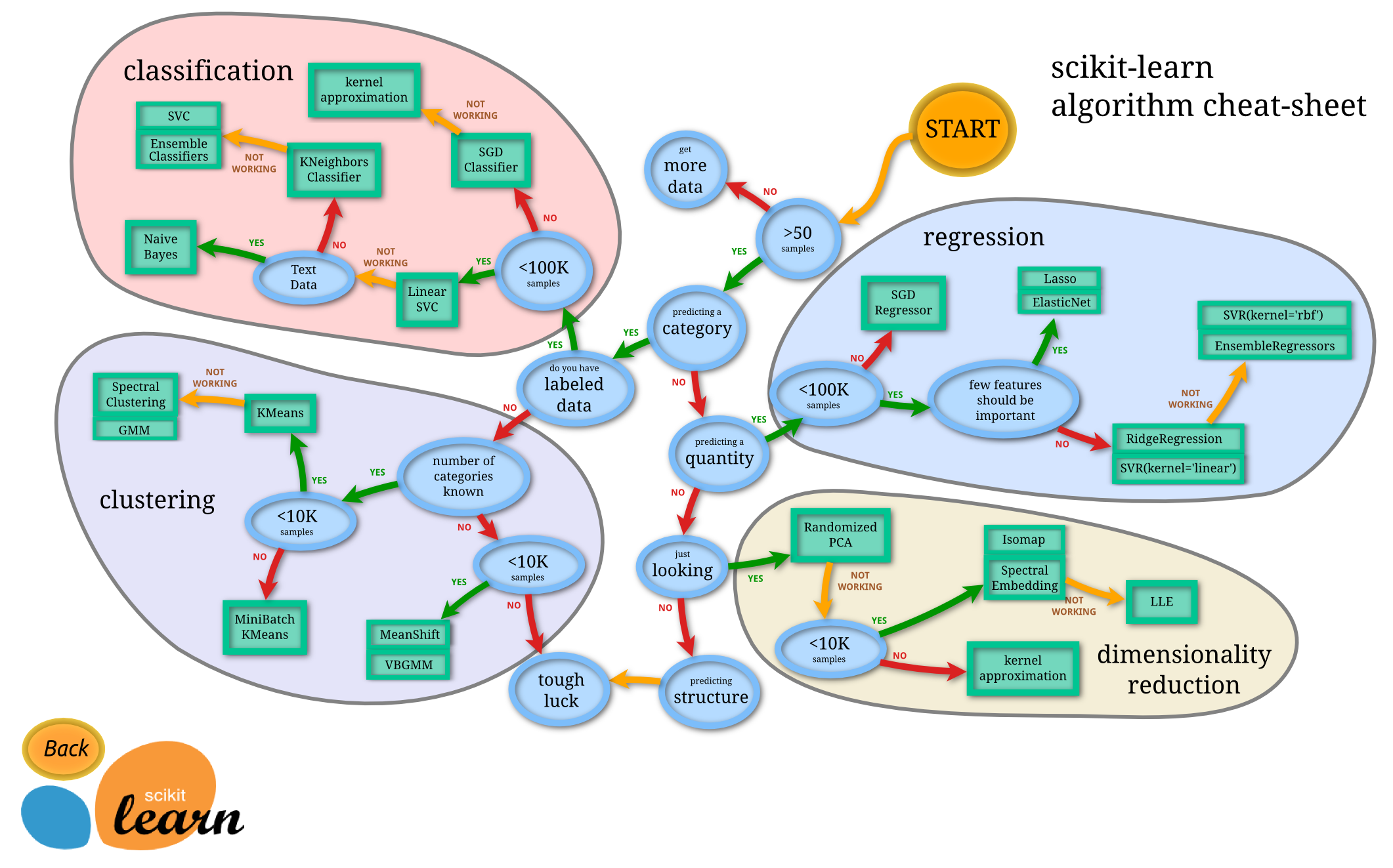
Cheat Sheet

from IPython.display import Image
Image("http://scikit-learn.org/dev/_static/ml_map.png", width=600)

Estimators

Given a scikit-learn estimator object named model, the following methods are available:

Available in all Estimators
- model.fit(): 训练数据。For supervised learning applications, this accepts two arguments: the data X and the labels y (e.g. model.fit(X, y)). For unsupervised learning applications, this accepts only a single argument, the data X (e.g. model.fit(X)).
Available in supervised estimators
- model.predict() : 预测。given a trained model, predict the label of a new set of data. This method accepts one argument, the new data X_new (e.g. model.predict(X_new)), and returns the learned label for each object in the array.
- model.predict_proba() : 预测概率。For classification problems, some estimators also provide this method, which returns the probability that a new observation has each categorical label. In this case, the label with the highest probability is returned by model.predict().
- model.score() : 评价模型。 for classification or regression problems, most (all?) estimators implement a score method. Scores are between 0 and 1, with a larger score indicating a better fit.
Available in unsupervised estimators
- model.predict() : predict labels in clustering algorithms.
- model.transform() : given an unsupervised model, transform new data into the new basis. This also accepts one argument X_new, and returns the new representation of the data based on the unsupervised model.
- model.fit_transform() : some estimators implement this method, which more efficiently performs a fit and a transform on the same input data.

2. 数据集Iris

from sklearn.datasets import load_iris
iris = load_iris()
n_samples, n_features = iris.data.shape
print(iris.keys())
print((n_samples, n_features))
print(iris.data.shape)
print(iris.target.shape)
print(iris.target_names)
print(iris.feature_names)

['target_names', 'data', 'target', 'DESCR', 'feature_names']
(150, 4)
(150, 4)
(150,)
['setosa' 'versicolor' 'virginica']
['sepal length (cm)', 'sepal width (cm)', 'petal length (cm)', 'petal width (cm)']

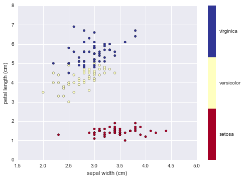
# sepal width
x_index = 1
# petal length
y_index = 2
formatter = plt.FuncFormatter(lambda i, *args: iris.target_names[int(i)])
plt.scatter(iris.data[:, x_index], iris.data[:, y_index],
            c=iris.target, cmap=plt.cm.get_cmap('RdYlBu', 3))
plt.colorbar(ticks=[0,1,2],format=formatter)
plt.clim(-0.5,2.5) # color limit
plt.xlabel(iris.feature_names[x_index])
plt.ylabel(iris.feature_names[y_index])
plt.show()

3. K-Nearest Neighbors Classifier

The K-Nearest Neighbors (KNN) algorithm is a method used for algorithm used for classification or for regression. In both cases, the input consists of the k closest training examples in the feature space. Given a new, unknown observation, look up which points have the closest features and assign the predominant class.

from sklearn import neighbors, datasets
iris = datasets.load_iris()
X, y = iris.data, iris.target
# new model
knn = neighbors.KNeighborsClassifier(n_neighbors=5,weights='uniform')
# fit model
knn.fit(X,y)
# example
X_pred = [3,5,4,2]
res = knn.predict([X_pred,])

print iris.target_names[res]
print iris.target_names
print knn.predict_proba([X_pred,])

['versicolor']
['setosa' 'versicolor' 'virginica']
[[ 0.   0.8  0.2]]

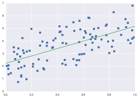
4. Linear Regression

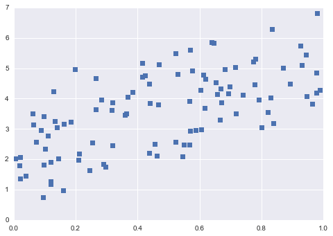
Linear Regression is a supervised learning algorithm that models the relationship between a scalar dependent variable y and one or more explanatory variables (or independent variable) denoted X.

from sklearn.linear_model import LinearRegression

np.random.seed(0)
X = np.random.random(size=(100,1))
y = 3 * X.squeeze() + 2 + np.random.randn(100)
plt.plot(X.squeeze(),y,'s')
plt.show()

model = LinearRegression()
model.fit(X,y)
# plot predicted data
X_fit = np.linspace(0,1,100).reshape(-1,1)
y_fit = model.predict(X_fit)
plt.plot(X.squeeze(),y,'s')
plt.plot(X_fit.squeeze(),y_fit)
plt.show()

/usr/local/lib/python2.7/site-packages/scipy/linalg/basic.py:884: RuntimeWarning: internal gelsd driver lwork query error, required iwork dimension not returned. This is likely the result of LAPACK bug 0038, fixed in LAPACK 3.2.2 (released July 21, 2010). Falling back to 'gelss' driver.
  warnings.warn(mesg, RuntimeWarning)

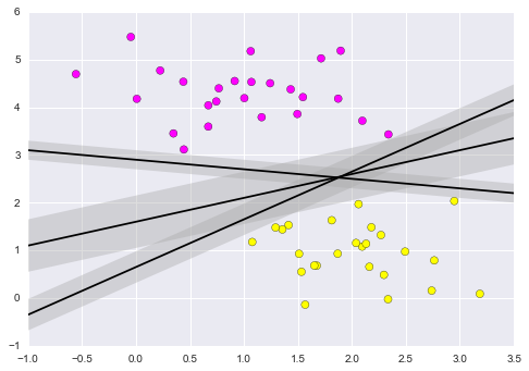
5. Support Vector Machine Classifier

Support Vector Machines (SVMs) are a powerful supervised learning algorithm used for classification or for regression. SVMs draw a boundary between clusters of data. SVMs attempt to maximize the margin between sets of points. Many lines can be drawn to separate the points above:

from sklearn.datasets.samples_generator import make_blobs
X,y = make_blobs(n_samples=50,centers=2,random_state=0,cluster_std=0.6)
xfit = np.linspace(-1,3.5)
plt.scatter(X[:,0],X[:,1],c=y,s=50,cmap='spring')
# draw lines
for m,b,d in [(1, 0.65, 0.33), (0.5, 1.6, 0.55), (-0.2, 2.9, 0.2)]:
    yfit = m*xfit + b
    plt.plot(xfit,yfit,'-k')
    plt.fill_between(xfit,yfit-d, yfit+d, edgecolor='none',color='#AAAAAA',alpha=0.4)
plt.xlim(-1,3.5);

Fit the model

from sklearn.svm import SVC
clf = SVC(kernel='linear')
clf.fit(X, y)

SVC(C=1.0, cache_size=200, class_weight=None, coef0=0.0,
  decision_function_shape=None, degree=3, gamma='auto', kernel='linear',
  max_iter=-1, probability=False, random_state=None, shrinking=True,
  tol=0.001, verbose=False)

Density Estimation: Gaussian Mixture Models

Here we'll explore Gaussian Mixture Models, which is an unsupervised clustering & density estimation technique.

Introducing Gaussian Mixture Models

We previously saw an example of K-Means, which is a clustering algorithm which is most often fit using an expectation-maximization approach.

Here we'll consider an extension to this which is suitable for both clustering and density estimation.

For example, imagine we have some one-dimensional data in a particular distribution:

np.random.seed(2)
x = np.concatenate([np.random.normal(0, 2, 2000),
                    np.random.normal(5, 5, 2000),
                    np.random.normal(3, 0.5, 600)])
plt.hist(x,bins=80,normed=True)
plt.xlim(-10,20);

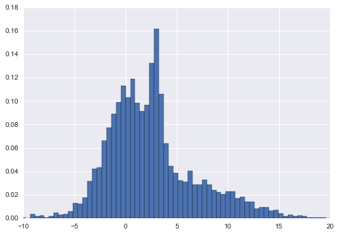
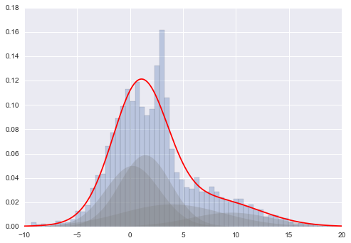
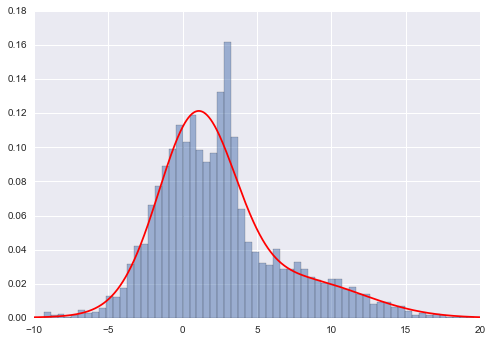
Gaussian mixture models will allow us to approximate this density:

x = x.reshape((-1,1))
from sklearn.mixture import GMM
# GMM.fit() Estimate model parameters with the EM algorithm.
clf = GMM(4,n_iter=500,random_state=3).fit(x)
xpdf = np.linspace(-10, 20, 1000).reshape((-1,1))
density = np.exp(clf.score(xpdf))

plt.hist(x[:,0], 80, normed=True, alpha=0.5)
plt.plot(xpdf, density, '-r')
plt.xlim(-10, 20);

plt.hist(x, 80, normed=True, alpha=0.3)
plt.plot(xpdf, density, '-r')

for i in range(clf.n_components):
    pdf = clf.weights_[i] * stats.norm(clf.means_[i, 0],
                                       np.sqrt(clf.covars_[i, 0])).pdf(xpdf)
    plt.fill(xpdf, pdf, facecolor='gray',
             edgecolor='none', alpha=0.3)
plt.xlim(-10, 20);

笔记2