一维最优化
scipy.optimize.minimize_scalar(更一般的接口)或scipy.optimize.brent(),参数见scipy.optimize.brent(func, args=(), brack=None, tol=1.48e-08, full_output=0, maxiter=500),主要是传入一个一维函数以及一个区间,然后返回最值。
例子
Brent’s method on a quadratic function: it converges in 3 iterations, as the quadratic approximation is then exact.
Brent’s method on a non-convex function: note that the fact that the optimizer avoided the local minimum is a matter of luck.
import numpy as np
from scipy import optimize as opt
def f(x):
    return -np.exp(-(x - .7)**2)
x_min = opt.brent(f)  # It actually converges in 9 iterations!
x_min

x_min - .7
-2.160590595323697e-10
基于梯度的算法
梯度下降法
Gradient descent basically consists in taking small steps in the direction of the gradient, that is the direction of the steepest descent.
共轭梯度法
梯度下降法有缺陷,遇到变化剧烈的地方,就会反复震荡,共轭梯度下降法解决这个问题。
The gradient descent algorithms above are toys not to be used on real problems.As can be seen from the above experiments, one of the problems of the simple gradient descent algorithms, is that it tends to oscillate across a valley, each time following the direction of the gradient, that makes it cross the valley. The conjugate gradient solves this problem by adding a friction term: each step depends on the two last values of the gradient and sharp turns are reduced.
Methods based on conjugate gradient are named with ‘cg’ in scipy. The simple conjugate gradient method to minimize a function is scipy.optimize.fmin_cg()
例子
def f(x):   # The rosenbrock function
    return .5*(1 - x[0])**2 + (x[1] - x[0]**2)**2
opt.fmin_cg(f, [2, 2])
Optimization terminated successfully.
         Current function value: 0.000000
         Iterations: 13
         Function evaluations: 120
         Gradient evaluations: 30


array([ 0.99998968,  0.99997855])
算法会自动计算根据函数计算导数梯度等,但如果传入导数计算会更快一些。
def fprime(x):
    return np.array((-2*.5*(1 - x[0]) - 4*x[0]*(x[1] - x[0]**2), 2*(x[1] - x[0]**2)))
opt.fmin_cg(f, [2, 2], fprime=fprime)
Optimization terminated successfully.
         Current function value: 0.000000
         Iterations: 13
         Function evaluations: 30
         Gradient evaluations: 30


array([ 0.99999199,  0.99998336])
牛顿法
Newton methods: using the Hessian (2nd differential)
Newton methods use a local quadratic approximation to compute the jump direction. For this purpose, they rely on the 2 first derivative of the function: the gradient and the Hessian.
In scipy, the Newton method for optimization is implemented in scipy.optimize.fmin_ncg() (cg here refers to that fact that an inner operation, the inversion of the Hessian, is performed by conjugate gradient).
例子
def f(x):   # The rosenbrock function
    return .5*(1 - x[0])**2 + (x[1] - x[0]**2)**2
def fprime(x):
    return np.array((-2*.5*(1 - x[0]) - 4*x[0]*(x[1] - x[0]**2), 2*(x[1] - x[0]**2)))
opt.fmin_ncg(f, [2, 2], fprime=fprime)
Optimization terminated successfully.
         Current function value: 0.000000
         Iterations: 9
         Function evaluations: 11
         Gradient evaluations: 51
         Hessian evaluations: 0


array([ 1.,  1.])
Note that compared to a conjugate gradient (above), Newton’s method has required less function evaluations, but more gradient evaluations, as it uses it to approximate the Hessian. Let’s compute the Hessian and pass it to the algorithm:
def hessian(x): # Computed with sympy
    return np.array(((1 - 4*x[1] + 12*x[0]**2, -4*x[0]), (-4*x[0], 2)))
opt.fmin_ncg(f, [2, 2], fprime=fprime, fhess=hessian)
Optimization terminated successfully.
         Current function value: 0.000000
         Iterations: 9
         Function evaluations: 11
         Gradient evaluations: 19
         Hessian evaluations: 9


array([ 1.,  1.])
全局最优化
If your problem does not admit a unique local minimum (which can be hard to test unless the function is convex), and you do not have prior information to initialize the optimization close to the solution, you may need a global optimizer.
Brute force: a grid search
scipy.optimize.brute() evaluates the function on a given grid of parameters and returns the parameters corresponding to the minimum value. The parameters are specified with ranges given to numpy.mgrid. By default, 20 steps are taken in each direction:
def f(x):   # The rosenbrock function
    return .5*(1 - x[0])**2 + (x[1] - x[0]**2)**2
opt.brute(f, ((-1, 2), (-1, 2)))
array([ 1.00001462, 1.00001547])
有约束最优化
As an example, let us consider the problem of maximizing the function: $f(x, y) = 2 x y + 2 x - x^2 - 2 y^2$ subject to an equality and an inequality constraints defined as: $\begin{eqnarray} x^3 - y &= 0 \ y - 1 &\geq 0 \end{eqnarray}$.
the objective function and its derivative are defined as follows.
def func(x, sign=1.0):
    """ Objective function """
    return sign*(2*x[0]*x[1] + 2*x[0] - x[0]**2 - 2*x[1]**2)
def func_deriv(x, sign=1.0):
    """ Derivative of objective function """
    dfdx0 = sign*(-2*x[0] + 2*x[1] + 2)
    dfdx1 = sign*(2*x[0] - 4*x[1])
    return np.array([ dfdx0, dfdx1 ])
Note that since minimize only minimizes functions, the sign parameter is introduced to multiply the objective function (and its derivative) by -1 in order to perform a maximization.
Then constraints are defined as a sequence of dictionaries, with keys type, fun and jac.
cons = ({'type': 'eq',
         'fun' : lambda x: np.array([x[0]**3 - x[1]]),
         'jac' : lambda x: np.array([3.0*(x[0]**2.0), -1.0])},
        {'type': 'ineq',
         'fun' : lambda x: np.array([x[1] - 1]),
         'jac' : lambda x: np.array([0.0, 1.0])})
- Now an unconstrained optimization can be performed as:
res = opt.minimize(func, [-1.0,1.0], args=(-1.0,), jac=func_deriv,
               method='SLSQP', options={'disp': True})
print(res.x)
Optimization terminated successfully.    (Exit mode 0)
            Current function value: -2.0
            Iterations: 4
            Function evaluations: 5
            Gradient evaluations: 4
[ 2.  1.]
- and a constrained optimization as:
res = opt.minimize(func, [-1.0,1.0], args=(-1.0,), jac=func_deriv,
               constraints=cons, method='SLSQP', options={'disp': True})
print res.x
Optimization terminated successfully.    (Exit mode 0)
            Current function value: -1.00000018311
            Iterations: 9
            Function evaluations: 14
            Gradient evaluations: 9
[ 1.00000009  1.        ]
线性拟合
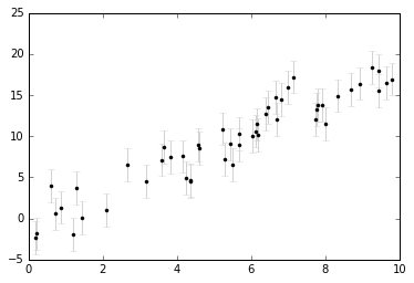
造数据
import matplotlib.pyplot as plt
%matplotlib inline
N = 50
m_true = 2
b_true = -1
dy = 2.0

np.random.seed(0)
xdata = 10 * np.random.random(N)
ydata = np.random.normal(b_true + m_true * xdata, dy)

plt.errorbar(xdata, ydata, dy,
             fmt='.k', ecolor='lightgray');
方法一: Using scipy.optimize.minimize
def chi2(theta, x, y):
    return np.sum(((y - theta[0] - theta[1] * x)) ** 2)
theta_guess = [0, 1]
theta_best = opt.fmin(chi2, theta_guess, args=(xdata, ydata))
print(theta_best)
Optimization terminated successfully.
         Current function value: 171.105514
         Iterations: 70
         Function evaluations: 129
[-1.01441373  1.93854462]
theta_guess = [0, 1]
theta_best = opt.minimize(chi2, theta_guess, args=(xdata, ydata)).x
print(theta_best)
[-1.0144199 1.93854654]
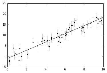
xfit = np.linspace(0, 10)
yfit = theta_best[0] + theta_best[1] * xfit

plt.errorbar(xdata, ydata, dy,
             fmt='.k', ecolor='lightgray');
plt.plot(xfit, yfit, '-k');
方法二: Least Squares Fitting
def deviations(theta, x, y):
    return (y - theta[0] - theta[1] * x)

theta_best, ier = opt.leastsq(deviations, theta_guess, args=(xdata, ydata))
print(theta_best)
[-1.01442017 1.93854659]
yfit = theta_best[0] + theta_best[1] * xfit

plt.errorbar(xdata, ydata, dy,
             fmt='.k', ecolor='lightgray');
plt.plot(xfit, yfit, '-k');

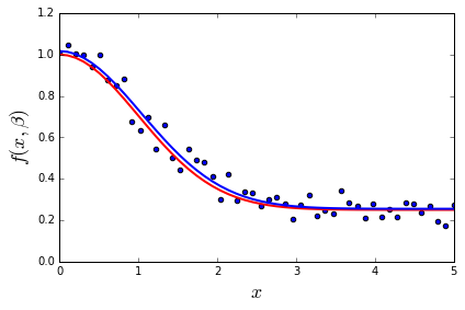
非线性拟合
def f(x, beta0, beta1, beta2):
    return beta0 + beta1 * np.exp(-beta2 * x**2)

beta = (0.25, 0.75, 0.5)
xdata = np.linspace(0, 5, 50)
y = f(xdata, *beta)
ydata = y + 0.05 * np.random.randn(len(xdata))

def g(beta):
    return ydata - f(xdata, *beta)

beta_start = (1, 1, 1)
beta_opt, beta_cov = opt.leastsq(g, beta_start)
beta_opt
array([ 0.25493905, 0.76190464, 0.46526094])
fig, ax = plt.subplots()
ax.scatter(xdata, ydata)
ax.plot(xdata, y, 'r', lw=2)
ax.plot(xdata, f(xdata, *beta_opt), 'b', lw=2)
ax.set_xlim(0, 5)
ax.set_xlabel(r"$x$", fontsize=18)
ax.set_ylabel(r"$f(x, \beta)$", fontsize=18)
fig.tight_layout()
beta_opt, beta_cov = opt.curve_fit(f, xdata, ydata)
beta_opt
array([ 0.25493905, 0.76190464, 0.46526094])