作业
- 学习理解如何使用最小二乘法的矩阵公式来得到线性回归的解,并用NumPy库实现该算法
- 使用pandas库函数,下载上证综指和任意一份成分股票数据,计算日收益率,对这两组数据建立回归模型,将上证综指的收益率作为解释变量,说明这个模型的用处
- 在kaggle网站上找到titanic数据,并使用logistic回归模型来建模,研究每个因素对生存的重要性
- 搜索某个城市过去一个月的PM2.5小时级数据,根据时间序列预测方法,来预测未来三天的PM2.5情况
import statsmodels.api as sm
import statsmodels.formula.api as smf
import statsmodels.graphics.api as smg
import patsy
%matplotlib inline
import matplotlib.pyplot as plt
import numpy as np
import pandas as pd
import seaborn as sns
from datetime import datetime
最小二乘法
学习理解如何使用最小二乘法的矩阵公式来得到线性回归的解,并用NumPy库实现该算法
0. 算例数据
np.random.seed(123456789)
y = np.array([1, 2, 3, 4, 5])
x1 = np.array([6, 7, 8, 9, 10])
x2 = np.array([11, 12, 13, 14, 15])
X = np.vstack([np.ones(5), x1, x2, x1*x2]).T
X
array([[   1.,    6.,   11.,   66.],
       [   1.,    7.,   12.,   84.],
       [   1.,    8.,   13.,  104.],
       [   1.,    9.,   14.,  126.],
       [   1.,   10.,   15.,  150.]])
1. 用statsmodel.api.OLS
model = sm.OLS(y, X)
result = model.fit()
result.params
array([ -5.55555556e-01,   1.88888889e+00,  -8.88888889e-01,
        -4.99600361e-16])
2. 用statsmodels.formula.api.ols
用DataFrame传入数据
data = {"y": y, "x1": x1, "x2": x2}
df_data = pd.DataFrame(data)
model = smf.ols("y ~ 1 + x1 + x2 + x1:x2", df_data)
result = model.fit()
result.params
Intercept   -5.555556e-01
x1           1.888889e+00
x2          -8.888889e-01
x1:x2       -4.996004e-16
dtype: float64
3. 用Numpy求解
numpy库提供了numpy.lstsq函数来求解最小二乘法。
beta, res, rank, sval = np.linalg.lstsq(X, y)
beta
array([ -5.55555556e-01,   1.88888889e+00,  -8.88888889e-01,
        -5.25467605e-16])
最小二乘法的公式特别简单,也可以直接用公式计算得出相应的系数
一元线性回归

多元线性回归

建立回归模型
使用pandas库函数,下载上证综指和任意一份成分股票数据,计算日收益率,对这两组数据建立回归模型,将上证综指的收益率作为解释变量,说明这个模型的用处。
数据获取及收益率计算
from pandas_datareader import data
import pandas as pd
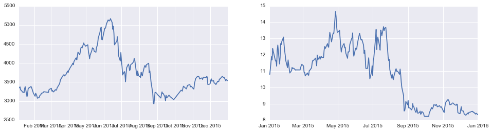
sh = data.DataReader("000001.SS", 'yahoo', '2015-1-1', '2016-1-1') # 上证综指
zsy = data.DataReader("601857.SS", 'yahoo', '2015-1-1', '2016-1-1') # 中石油
fig,(ax1,ax2) = plt.subplots(1,2,figsize=(16,4))
ax1.plot(sh.Close)
ax2.plot(zsy.Close)
plt.show()
# accept stock price and return series back
def get_rs(price):
    return np.log((price.shift(1)/price).dropna())
rs_sh = get_rs(sh.Close) # return series
rs_zsy = get_rs(zsy.Close)
整理数据
由于两者数据不完全对应,比如有的日期上证综指没数据,而中石油有,所以取数据的交集
print rs_sh.shape
print rs_zsy.shape
(232,)
(261,)
index = rs_sh.index.intersection(rs_zsy.index)
index.shape
(232,)
rs_sh = rs_sh[index]
rs_zsy = rs_zsy[index]
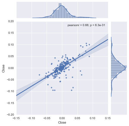
可视化
可以画图看其相关性,从regression plot来看,其相关性还是很明显的。
sns.jointplot(rs_sh,rs_zsy, kind="reg");
回归
以上证综指为自变量,中石油为因变量做regression,用smf.ols实现该回归。
data = {"y": rs_zsy, "x": rs_sh}
df = pd.DataFrame(data)
model = smf.ols("y ~ 1 + x ", df)
result = model.fit()
result.params
Intercept    0.001824
x            0.802182
dtype: float64
print result.summary()
                            OLS Regression Results
==============================================================================
Dep. Variable:                      y   R-squared:                       0.442
Model:                            OLS   Adj. R-squared:                  0.439
Method:                 Least Squares   F-statistic:                     181.8
Date:                Sun, 19 Jun 2016   Prob (F-statistic):           6.35e-31
Time:                        21:55:42   Log-Likelihood:                 547.09
No. Observations:                 232   AIC:                            -1090.
Df Residuals:                     230   BIC:                            -1083.
Df Model:                           1
Covariance Type:            nonrobust
==============================================================================
                 coef    std err          t      P>|t|      [95.0% Conf. Int.]
------------------------------------------------------------------------------
Intercept      0.0018      0.002      1.208      0.228        -0.001     0.005
x              0.8022      0.059     13.484      0.000         0.685     0.919
==============================================================================
Omnibus:                      108.491   Durbin-Watson:                   2.056
Prob(Omnibus):                  0.000   Jarque-Bera (JB):              595.222
Skew:                          -1.788   Prob(JB):                    5.61e-130
Kurtosis:                       9.984   Cond. No.                         39.4
==============================================================================

Warnings:
[1] Standard Errors assume that the covariance matrix of the errors is correctly specified.
逻辑回归
在kaggle网站上找到titanic数据,并使用logistic回归模型来建模,研究每个因素对生存的重要性
数据清理
!ls data/
genderclassmodel.csv test.csv
gendermodel.csv      train.csv
df = pd.read_csv('data/train.csv',index_col='PassengerId') # id is unique
df.head(3)
| Survived | Pclass | Name | Sex | Age | SibSp | Parch | Ticket | Fare | Cabin | Embarked | |
|---|---|---|---|---|---|---|---|---|---|---|---|
| PassengerId | |||||||||||
| 1 | 0 | 3 | Braund, Mr. Owen Harris | male | 22.0 | 1 | 0 | A/5 21171 | 7.2500 | NaN | S |
| 2 | 1 | 1 | Cumings, Mrs. John Bradley (Florence Briggs Th... | female | 38.0 | 1 | 0 | PC 17599 | 71.2833 | C85 | C |
| 3 | 1 | 3 | Heikkinen, Miss. Laina | female | 26.0 | 0 | 0 | STON/O2. 3101282 | 7.9250 | NaN | S |
df.Survived.value_counts()
0    549
1    342
Name: Survived, dtype: int64
df.Sex = df.Sex.map({'male': 0, 'female':1}) # map category to num to be better explained
df.isnull().sum()
Survived      0
Pclass        0
Name          0
Sex           0
Age         177
SibSp         0
Parch         0
Ticket        0
Fare          0
Cabin       687
Embarked      2
dtype: int64
Cabin列数据缺失太多,舍弃之,并drop NaN
df = df.drop(['Ticket', 'Cabin'], axis=1)
df = df.dropna()
df.isnull().any() # 数据比较干净
Survived    False
Pclass      False
Name        False
Sex         False
Age         False
SibSp       False
Parch       False
Fare        False
Embarked    False
dtype: bool
df.head(2)
| Survived | Pclass | Name | Sex | Age | SibSp | Parch | Fare | Embarked | |
|---|---|---|---|---|---|---|---|---|---|
| PassengerId | |||||||||
| 1 | 0 | 3 | Braund, Mr. Owen Harris | 0 | 22.0 | 1 | 0 | 7.2500 | S |
| 2 | 1 | 1 | Cumings, Mrs. John Bradley (Florence Briggs Th... | 1 | 38.0 | 1 | 0 | 71.2833 | C |
数据基本解读及可视化
- PassengerId: 乘客的id,是unique的。
- Survived:生存与否。0 = No,1 = Yes这是我们建模的目标变量。
- Pclass:客舱等级,1 = 1st; 2 = 2nd; 3 = 3rd,1st代表头等舱。可以反映一个人的经济地位,可能对模型的预测有贡献。
- Name: 姓名
- Sex: 性别, contribute a lot, 从电影里我们也知道,女人存活的几率更大。
- Age: 年龄, 女人与小孩先走,可以猜测,年龄也是一个很重要的因素。
- SibSp: 亲属人数,Number of Siblings/Spouses Aboard。
- Parch: 父母或子女数,即Number of Parents/Children Aboard。
- Fare: 船票价格。
- Cabin: 客舱。
- Embarked: 即Port of Embarkation,登船港口。C = Cherbourg(瑟堡,法国); Q = Queenstown(昆士城,新加坡); S = Southampton(南安普顿,英国)
从已有信息判断,乘客的性别,年龄以及客舱等级是比较重要的因素,建模时候要优先考虑。同时,基于数据挖掘的理念,我们当然要考虑其他因素的贡献啦!接下来就探究各个变量的对模型预测的贡献。
数据分布
fig = plt.figure(figsize=(18,6),dpi=1600)
alpha = alpha_scatterplot = 0.2
alpha_bar_chart = 0.55

# 把各个图放在一个grid画布上 subplot2grid
# 生VS死
ax1 = plt.subplot2grid((2,3),(0,0))
# Series.values, Series.value_counts()
df.Survived.value_counts().plot.bar(alpha=alpha_bar_chart) # or plot(kind='bar)
ax1.set_xlim(-1,2)
ax1.set_title('Distribution of Survival, (1 = Survived)')

# survive by age
ax2 = plt.subplot2grid((2,3),(0,1))
ax2.scatter(df.Survived, df.Age, alpha=alpha_scatterplot)
ax2.set_ylabel('Age')
ax2.grid(b=True,which='major',axis='y')
ax2.set_title("Survival by Age,  (1 = Survived)")

# class distribution
ax3 = plt.subplot2grid((2,3),(0,2))
df.Pclass.value_counts().plot.barh(alpha=alpha_bar_chart)
ax3.set_ylim(-1,len(df.Pclass.value_counts()))
ax3.set_title('Class Distribution')

# plot kernel density estimate passangers's age by class
# get to know the distribution of age within class
ax4 = plt.subplot2grid((2,3),(1,0),colspan=2)
df.Age[df.Pclass==1].plot.kde()
df.Age[df.Pclass==2].plot.kde()
df.Age[df.Pclass==3].plot.kde()
ax4.set_xlabel('Age')
ax4.set_title('Age Distribution within classes')
ax4.legend(('1st Class', '2nd Class','3rd Class'),loc='best')

ax5 = plt.subplot2grid((2,3),(1,2))
df.Embarked.value_counts().plot.bar(alpha=alpha_bar_chart)
ax5.set_xlim(-1, len(df.Embarked.value_counts()))
ax5.set_title("Passengers per boarding location")

plt.show()
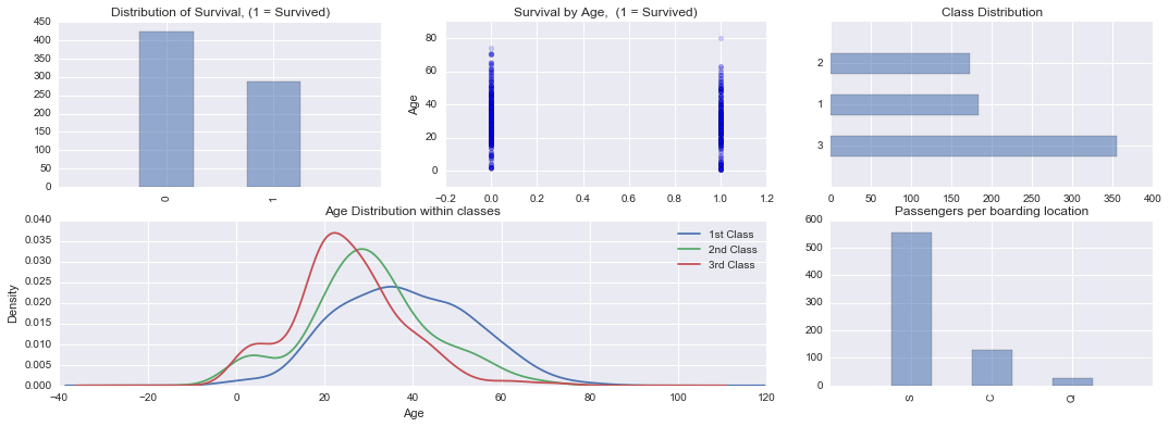
从图中可以看出生存分布等一系列信息,比如Survival by Age可以看出,幸存者的年龄明显偏低,遇难者的年龄明显偏高,从Age Distribution within classes可以看出一个有趣的现象,就是坐头等舱的人年龄偏大,经济舱的年龄偏小,还是多混几年有钱哈哈!
幸存率分解
fig = plt.figure(figsize=(18,4), dpi=1600)
ax1=fig.add_subplot(141)
female_highclass = df.Survived[df.Sex == 1][df.Pclass != 3].value_counts(sort=False)
female_highclass.plot(kind='bar', label='female, highclass', color='#FA2479', alpha=0.65)
ax1.set_xticklabels(["Died","Survived"], rotation=0)
ax1.set_xlim(-1, len(female_highclass))
plt.legend(loc='best')

ax2=fig.add_subplot(142, sharey=ax1)
female_lowclass = df.Survived[df.Sex == 1][df.Pclass == 3].value_counts(sort=False)
female_lowclass.plot(kind='bar', label='female, lowclass', color='pink', alpha=0.65)
ax2.set_xticklabels(["Died","Survived"], rotation=0)
ax2.set_xlim(-1, len(female_lowclass))
plt.legend(loc='best')

ax3=fig.add_subplot(143, sharey=ax1)
male_highclass = df.Survived[df.Sex == 0][df.Pclass != 3].value_counts(sort=False)
male_highclass.plot(kind='bar', label='male, highclass', alpha=0.65, color='steelblue')
ax3.set_xticklabels(["Died","Survived"], rotation=0)
ax3.set_xlim(-1, len(male_highclass))
plt.legend(loc='best')

ax4=fig.add_subplot(144, sharey=ax1)
male_lowclass = df.Survived[df.Sex == 0][df.Pclass == 3].value_counts(sort=False)
male_lowclass.plot(kind='bar', label='male, lowclass',color='lightblue', alpha=0.65)
ax4.set_xticklabels(["Died","Survived"], rotation=0)
ax4.set_xlim(-1, len(male_lowclass))
plt.legend(loc='best')

plt.show()

从上图中可以明显的看出,女性的幸存率明显偏高,同时在highclass客舱的乘客,存活几率更高。一个粗暴的结论,贵族女性幸存几率极大!
逻辑回归分析
图示还不够严谨,让我们用逻辑回归来分析各个因素对生存的影响。我们先逐一地对各个因素做逻辑回归,得到感兴趣的参数,然后决定最终的参数。
model = smf.logit('Survived ~ C(Sex) + Age + C(Pclass) + SibSp + Parch + Fare', data=df)
result = model.fit(disp=0)
print result.summary()
由于result.summary()给出的参数太过于丰富,这里自定义一个简单的函数,只提取伪R^2,pvalue以及系数。伪R^2是coefficient of determination R^2的一个alternative,反映了该变量对目标变量的贡献;pvalue反映了其统计属性,如果足够小,有理由认为是统计显著的,而不是随机因素引起的;系数值的正负也很关键。
def log_it(formula):
    # fit model, get psudo rsquare, pvalue and param
    model = smf.logit(formula,data=df)
    result = model.fit(disp=0) # compress unnecessary output
    return result.prsquared, result.pvalues[-1],result.params[-1]
据我们现有的信息,Sex与Pclass是比较重要的因素,只需要额外考虑其他几个因素的影响,当然有的变量比如Name明显不适合拿来做预测,所以也不考虑。
names = ['Age', 'SibSp', 'Parch', 'Fare','C(Embarked)']
for name in names:
    formula = "Survived ~ C(Sex) + C(Pclass) + " + str(name)
    print name, log_it(formula)
Age (0.32699736957050418, 1.236270259598232e-06, -0.037194172532429647)
SibSp (0.30370496630664234, 0.091433654690944763, -0.19335798881357269)
Parch (0.3010825162811821, 0.49539569705080821, -0.073802940746361581)
Fare (0.30158076955799806, 0.3438308520558121, 0.0021622693143560417)
C(Embarked) (0.30677909012802962, 0.021998776007212204, -0.58969578190897542)
从回归结果看:
- Age,Embarked与SibSp贡献的比例比较高,其对应的伪R^2(包含Sex于Pclass)比较高,分别是0.326997,0.306779,0.303705,我们认为这是比较重要的因素。
- 而且除了SibSP以外,Age与Embarked对用的pvalue也比较小,也就是统计意义上显著的,不大可能是因为随机因素造成的。
- 在看其系数,Age的系数为负,意味着年龄越小,越有可能幸存;其他因素类似。
回归建模
model = smf.logit('Survived ~ C(Sex) + C(Pclass)  + Age + SibSp + C(Embarked)', data=df)
result = model.fit(disp=False)
print result.summary()
                           Logit Regression Results
==============================================================================
Dep. Variable:               Survived   No. Observations:                  712
Model:                          Logit   Df Residuals:                      704
Method:                           MLE   Df Model:                            7
Date:                Sun, 19 Jun 2016   Pseudo R-squ.:                  0.3414
Time:                        21:55:44   Log-Likelihood:                -316.40
converged:                       True   LL-Null:                       -480.45
                                        LLR p-value:                 5.992e-67
====================================================================================
                       coef    std err          z      P>|z|      [95.0% Conf. Int.]
------------------------------------------------------------------------------------
Intercept            1.9184      0.420      4.570      0.000         1.096     2.741
C(Sex)[T.1]          2.6239      0.218     12.060      0.000         2.197     3.050
C(Pclass)[T.2]      -1.2673      0.299     -4.245      0.000        -1.852    -0.682
C(Pclass)[T.3]      -2.4966      0.296     -8.422      0.000        -3.078    -1.916
C(Embarked)[T.Q]    -0.8351      0.597     -1.398      0.162        -2.006     0.335
C(Embarked)[T.S]    -0.4254      0.271     -1.572      0.116        -0.956     0.105
Age                 -0.0436      0.008     -5.264      0.000        -0.060    -0.027
SibSp               -0.3697      0.123     -3.004      0.003        -0.611    -0.129
====================================================================================
模型加入Fare以及Parch等因素后,对伪R^2的提升很不明显,还有可能造成过拟合问题,所以目前只考虑如上因素。最终的伪R方是0.3414。
print result.get_margeff().summary()
        Logit Marginal Effects
=====================================
Dep. Variable:               Survived
Method:                          dydx
At:                           overall
====================================================================================
                      dy/dx    std err          z      P>|z|      [95.0% Conf. Int.]
------------------------------------------------------------------------------------
C(Sex)[T.1]          0.3733      0.017     21.918      0.000         0.340     0.407
C(Pclass)[T.2]      -0.1803      0.041     -4.422      0.000        -0.260    -0.100
C(Pclass)[T.3]      -0.3552      0.035    -10.046      0.000        -0.424    -0.286
C(Embarked)[T.Q]    -0.1188      0.085     -1.404      0.160        -0.285     0.047
C(Embarked)[T.S]    -0.0605      0.038     -1.581      0.114        -0.136     0.015
Age                 -0.0062      0.001     -5.619      0.000        -0.008    -0.004
SibSp               -0.0526      0.017     -3.066      0.002        -0.086    -0.019
====================================================================================
从回归结果看,依然是性别和客舱等级对幸存与否的影响更大。
模型评价
把因素考虑在一起建模得出的pvalues与单独建模的有点出入,比如单独建模时SibSp统计意义不显著,而综合建模其统计意义比较显著,还不清楚其理论解释,future work。
result.pvalues
Intercept           4.881669e-06
C(Sex)[T.1]         1.717358e-33
C(Pclass)[T.2]      2.184919e-05
C(Pclass)[T.3]      3.705960e-17
C(Embarked)[T.Q]    1.619715e-01
C(Embarked)[T.S]    1.160436e-01
Age                 1.408330e-07
SibSp               2.663272e-03
dtype: float64
预测评分
# read test data and combine them
df_test = pd.read_csv('data/test.csv',index_col="PassengerId")
df_survived = pd.read_csv('data/gendermodel.csv',index_col='PassengerId')
df_test['Survived'] = df_survived # 整合到一个DataFrame里便于操作
df_test.Sex = df_test.Sex.map({'female':1,'male':0})
df_test.head(3)
| Pclass | Name | Sex | Age | SibSp | Parch | Ticket | Fare | Cabin | Embarked | Survived | |
|---|---|---|---|---|---|---|---|---|---|---|---|
| PassengerId | |||||||||||
| 892 | 3 | Kelly, Mr. James | 0 | 34.5 | 0 | 0 | 330911 | 7.8292 | NaN | Q | 0 |
| 893 | 3 | Wilkes, Mrs. James (Ellen Needs) | 1 | 47.0 | 1 | 0 | 363272 | 7.0000 | NaN | S | 1 |
| 894 | 2 | Myles, Mr. Thomas Francis | 0 | 62.0 | 0 | 0 | 240276 | 9.6875 | NaN | Q | 0 |
df_test.drop(['Cabin'],axis=1,inplace=True)
df_test = df_test.dropna()
df_test['Survived_p'] = result.predict(df_test)
df_test.head(3)
| Pclass | Name | Sex | Age | SibSp | Parch | Ticket | Fare | Embarked | Survived | Survived_p | |
|---|---|---|---|---|---|---|---|---|---|---|---|
| PassengerId | |||||||||||
| 892 | 3 | Kelly, Mr. James | 0 | 34.5 | 0 | 0 | 330911 | 7.8292 | Q | 0 | 0.051230 |
| 893 | 3 | Wilkes, Mrs. James (Ellen Needs) | 1 | 47.0 | 1 | 0 | 363272 | 7.0000 | S | 1 | 0.309946 |
| 894 | 2 | Myles, Mr. Thomas Francis | 0 | 62.0 | 0 | 0 | 240276 | 9.6875 | Q | 0 | 0.052674 |
概率大于0.5的我们预测为幸存,记为1。
df_test['Survived_predict'] = (df_test['Survived_p'] > 0.5).astype(int)
df_test.head(3)
| Pclass | Name | Sex | Age | SibSp | Parch | Ticket | Fare | Embarked | Survived | Survived_p | Survived_predict | |
|---|---|---|---|---|---|---|---|---|---|---|---|---|
| PassengerId | ||||||||||||
| 892 | 3 | Kelly, Mr. James | 0 | 34.5 | 0 | 0 | 330911 | 7.8292 | Q | 0 | 0.051230 | 0 |
| 893 | 3 | Wilkes, Mrs. James (Ellen Needs) | 1 | 47.0 | 1 | 0 | 363272 | 7.0000 | S | 1 | 0.309946 | 0 |
| 894 | 2 | Myles, Mr. Thomas Francis | 0 | 62.0 | 0 | 0 | 240276 | 9.6875 | Q | 0 | 0.052674 | 0 |
predict = df_test['Survived'] == df_test['Survived_predict']
预测的幸存情况Survived_predict与实际的幸存情况对比,得出预测准确率。'Survived ~ C(Sex) + C(Pclass) + Age + SibSp + C(Embarked)'的预测效果还不错。
float(predict.sum())/len(predict)
0.9093655589123867
逻辑回归python实现
逻辑回归与线性回归类似,只不过有个logit函数的区别,用numpy库可以比较容易地实现,其中会用到梯度上升算法求解极大似然函数的最优值。
准备数据
提取用以训练和检验的数据,这里只考虑Pclass,Sex,Age,Fare四个维度。
X_train = np.array(df[['Pclass','Sex','Age','Fare']])
y_train = np.array(df['Survived']).reshape([-1,1])
X_test = np.array(df_test[['Pclass','Sex','Age','Fare']])
y_test = np.array(df_test['Survived']).reshape([-1,1])
sigmoid函数
定义sigmoid函数,因为线性回归的值范围落在[-oo,+oo],而概率范围为[0,1],sigmoid函数很好地把整个实数集map到零一区间。
def sigmoid(x):
    x = np.array(x)
    return 1.0/(1+np.exp(-x))
梯度上升算法
梯度上升算法(与梯度下降算法基本一致,只不过是求最大值),求解似然函数的最大值。
极大似然函数推导:

梯度:

迭代公式:

公式中的theta就是我们感兴趣的系数,是各个因素所占的权重。
def gradAsent(X,y,alpha = 0.001,niter = 1000):
    """
    X: X_train, train data with n features
    y: y_train, train data target
    """
    m, n = X.shape
    weights = np.ones((n,1))
    for i in range(niter):
        h = sigmoid(np.dot(X,weights))
        error = y - h
        weights = weights + alpha * np.dot(X.T,error)
    return weights
预测
接受与训练数据同样格式的数据,返回对应的目标变量,如果概率大于或等于0.5认为幸存,记为1,反之为0,所以数据已nparray形式操作。
def predict(X,weights):
    t = np.dot(X,weights)
    prob = sigmoid(t)
    res = (prob >= 0.5).astype(np.int)
    return res.flatten()
评价
预测准确率为67%,并不是特别理想,算法实现的比较基本,还需要一些润色,同时参数也有调优的余地。
weights = gradAsent(X_train,y_train)
res = predict(X_test,weights)
r = y_test.flatten() == res
float(r.sum())/len(r)
0.6706948640483383
随机森林
随机森林是一种比较新的机器学习模型。经典的机器学习模型是神经网络,有半个多世纪的历史了。神经网络预测精确,但是计算量很大。上世纪八十年代Breiman等人发明分类树的算法(Breiman et al. 1984),通过反复二分数据进行分类或回归,计算量大大降低。2001年Breiman把分类树组合成随机森林(Breiman 2001a),即在变量(列)的使用和数据(行)的使用上进行随机化,生成很多分类树,再汇总分类树的结果。随机森林在运算量没有显著提高的前提下提高了预测精度。随机森林对多元公线性不敏感,结果对缺失数据和非平衡的数据比较稳健,可以很好地预测多达几千个解释变量的作用(Breiman 2001b),被誉为当前最好的算法之一。
随机森林顾名思义,是用随机的方式建立一个森林,森林里面有很多的决策树组成,随机森林的每一棵决策树之间是没有关联的。在得到森林之后,当有一个新的输入样本进入的时候,就让森林中的每一棵决策树分别进行一下判断,看看这个样本应该属于哪一类(对于分类算法),然后看看哪一类被选择最多,就预测这个样本为那一类。
具体每棵树根据下列算法而建造:
- 用 N 来表示训练例子的个数,M表示变量的数目。
- 我们会被告知一个数 m ,被用来决定当在一个节点上做决定时,会使用到多少个变量。m应小于M
- 从N个训练案例中以可重复取样的方式,取样N次,形成一组训练集(即bootstrap取样)。并使用这棵树来对剩余预测其类别,并评估其误差。
- 对于每一个节点,随机选择m个基于此点上的变量。根据这 m 个变量,计算其最佳的分割方式。
- 每棵树都会完整成长而不会剪枝(Pruning)(这有可能在建完一棵正常树状分类器后会被采用)。
下图是来自wiki的一张小图。
from patsy import dmatrices
import sklearn.ensemble as ske # 随机森林在这个模块下
formula = 'Survived ~ C(Sex) + C(Pclass) + Age + SibSp + C(Embarked)'
# 构造我们需要的数据
y, x = dmatrices(formula, data=df, return_type='dataframe')
y.head(2)
| Survived | |
|---|---|
| PassengerId | |
| 1 | 0.0 |
| 2 | 1.0 |
x.head(2)
| Intercept | C(Sex)[T.1] | C(Pclass)[T.2] | C(Pclass)[T.3] | C(Embarked)[T.Q] | C(Embarked)[T.S] | Age | SibSp | |
|---|---|---|---|---|---|---|---|---|
| PassengerId | ||||||||
| 1 | 1.0 | 0.0 | 0.0 | 1.0 | 0.0 | 1.0 | 22.0 | 1.0 |
| 2 | 1.0 | 1.0 | 0.0 | 0.0 | 0.0 | 0.0 | 38.0 | 1.0 |
# 随机森林分类器需要一个一维数组,把DataFrame转换,利用ravel方法。
y = np.asarray(y).ravel()
results_rf = ske.RandomForestClassifier(n_estimators=100).fit(x, y)
# 平均准确率
score = results_rf.score(x, y)
score
0.9339887640449438
支持向量机
在机器学习中,支持向量机(SVM,还支持矢量网络)是与相关的学习算法有关的监督学习模型,可以分析数据,识别模式,用于分类和回归分析。给定一组训练样本,每个标记为属于两类,一个SVM训练算法建立了一个模型,分配新的实例为一类或其他类,使其成为非概率二元线性分类。一个SVM模型的例子,如在空间中的点,映射,使得所述不同的类别的例子是由一个明显的差距是尽可能宽划分的表示。新的实施例则映射到相同的空间中,并预测基于它们落在所述间隙侧上属于一个类别。 除了进行线性分类,支持向量机可以使用所谓的核技巧,它们的输入隐含映射成高维特征空间中有效地进行非线性分类。
支持向量机的基本思路是用一条超曲线或曲面,把不同类别的分开;同时不要数据太多的信任,让超曲线或曲面离边界最远。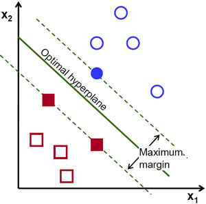
这里使用sklearn库里的函数实现,并使用不同的kernel作图比较效果。
from sklearn import datasets, svm
from sklearn import cross_validation
# create a regression friendly data frame
y, x = dmatrices(formula, data=df, return_type='matrix')

feature_1 = 2
feature_2 = 3
X = np.asarray(x)
X = X[:,[feature_1, feature_2]]

y = np.asarray(y)
# 我们需要一维数据,所以flatten一下
y = y.flatten().astype(np.float)

# 交叉验证
X_train, X_test, y_train, y_test = cross_validation.train_test_split(X, y, train_size=0.9,random_state=12345)

# 尝试不同的kernel
kernels = ['linear', 'rbf', 'poly']

color_map = plt.cm.Accent
fig,axes = plt.subplots(1,3,figsize=(14,4));
for fig_num, kernel in enumerate(kernels):
    clf = svm.SVC(kernel=kernel, gamma=3)
    clf.fit(X_train, y_train)

    axes[fig_num].scatter(X[:, 0], X[:, 1], c=y, zorder=10, cmap=color_map)

    # circle out the test data
    axes[fig_num].scatter(X_test[:, 0], X_test[:, 1], s=80, facecolors='none', zorder=10)

    x_min = X[:, 0].min(); x_max = X[:, 0].max()
    y_min = X[:, 1].min(); y_max = X[:, 1].max()

    XX, YY = np.mgrid[x_min:x_max:200j, y_min:y_max:200j]
    Z = clf.decision_function(np.c_[XX.ravel(), YY.ravel()])

    # put the result into a color plot
    Z = Z.reshape(XX.shape)
    axes[fig_num].pcolormesh(XX, YY, Z > 0, cmap=color_map)
    axes[fig_num].contour(XX, YY, Z, colors=['k', 'k', 'k'], linestyles=['--', '-', '--'],
               levels=[-.5, 0, .5])

    axes[fig_num].set_title(kernel)

建模
这里取ploy这一kernel建模,同时也可以调节gamma参数来改善模型的质量。
df_test.head(3)
| Pclass | Name | Sex | Age | SibSp | Parch | Ticket | Fare | Embarked | Survived | Survived_p | Survived_predict | |
|---|---|---|---|---|---|---|---|---|---|---|---|---|
| PassengerId | ||||||||||||
| 892 | 3 | Kelly, Mr. James | 0 | 34.5 | 0 | 0 | 330911 | 7.8292 | Q | 0 | 0.051230 | 0 |
| 893 | 3 | Wilkes, Mrs. James (Ellen Needs) | 1 | 47.0 | 1 | 0 | 363272 | 7.0000 | S | 1 | 0.309946 | 0 |
| 894 | 2 | Myles, Mr. Thomas Francis | 0 | 62.0 | 0 | 0 | 240276 | 9.6875 | Q | 0 | 0.052674 | 0 |
clf = svm.SVC(kernel='poly', gamma=3).fit(X_train, y_train)
y,x = dmatrices(formula, data=df_test, return_type='dataframe')
# 改变[1,3]的值,探究感兴趣的列
res_svm = clf.predict(x.ix[:,[1,3]].dropna())
res_svm = pd.DataFrame(res_svm,columns=['Survived'])
时间序列
搜索某个城市过去一个月的PM2.5小时级数据,根据时间序列预测方法,来预测未来三天的PM2.5情况。最初是从青悦开放数据中心获取的数据,但是遇到了奇奇怪怪的错误,不resample不能predict,resample之后不能fit,debug了好久还是放弃了Lol,这周浪太久,没时间折腾了,参考linmiao同学的数据,非常感谢。
数据清洗
pm = pd.read_csv('pm2_5.csv', header = None)
pm.head(3)
| 0 | 1 | 2 | 3 | 4 | |
|---|---|---|---|---|---|
| 0 | day | hour | avg | conc | city |
| 1 | 01/05/16 | 0 | 199 | 148 | 0 |
| 2 | 01/05/16 | 1 | 199 | 149 | 0 |
数据整理,把时间整合到一起,drop掉不需要的数据等。
pm.columns = pm.iloc[0,:]
pm = pm.drop(0)
pm.date = pm.day + ' ' + pm.hour + ':00:00'
pm['date'] = pm.date.apply(lambda x : datetime.strptime(x, '%d/%m/%y %H:%M:%S'))
pm = pm.set_index('date')
pm['avg'] = pm['avg'].astype(float)
pm = pm[['avg']]
pm.head(3)
| avg | |
|---|---|
| date | |
| 2016-05-01 00:00:00 | 199.0 |
| 2016-05-01 01:00:00 | 199.0 |
| 2016-05-01 02:00:00 | 204.0 |
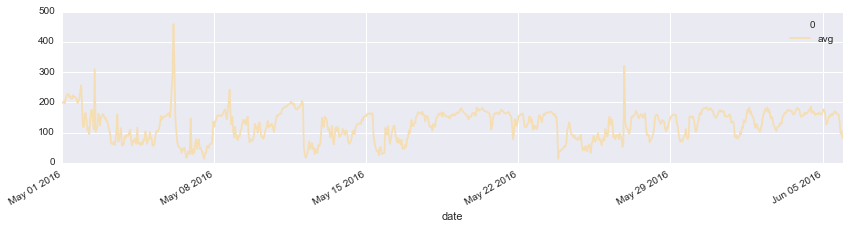
PM2.5近一个月的波动情况,除个别日子有异常值之外,可以看出pm2.5是一个比较平稳的时间序列。
pm.plot(figsize=(14,3),color='wheat');
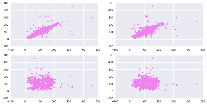
自相关探索
从下图可以看出,当lag比较小的时候,自相关还是比较明显的,但是当lag增加到24小时之后的时候,基本看不到相关性。
fig, axes = plt.subplots(2,2,figsize=(12,6))
axes[0][0].scatter(pm[1:], pm[:-1],color='violet');
axes[0][1].scatter(pm[2:], pm[:-2],color='violet');
axes[1][0].scatter(pm[24:], pm[:-24],color='violet');
axes[1][1].scatter(pm[48:], pm[:-48],color='violet');
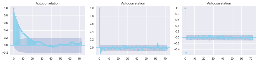
从下图一可以看出,pm2.5的自相关性随lag的增加递减,且呈现周期性,观察可以发现在24,48等处最弱。取一阶差分之后的自相关性已经很平稳了。
fig, axes = plt.subplots(1, 3, figsize=(12, 3))
smg.tsa.plot_acf(pm.avg, lags=72, ax=axes[0],color='skyblue')
smg.tsa.plot_acf(pm.avg.diff().dropna(), lags=72, ax=axes[1],color='skyblue')
smg.tsa.plot_acf(pm.avg.diff().diff().dropna(), lags=72, ax=axes[2],color='skyblue')
fig.tight_layout()
建模
建立Autoregressive AR(p)模型,拟合然后用以预测。
model = sm.tsa.AR(pm.avg)
result = model.fit(48)
检验残差是否存在自相关性
用sm.stats.durbin_watson(result.resid)实现。原假设是不存在自相关性。
The test statistic is approximately equal to 2*(1-r) where
ris the sample autocorrelation of the residuals. Thus, for r == 0, indicating no serial correlation, the test statistic equals 2. This statistic will always be between 0 and 4. The closer to 0 the statistic, the more evidence for positive serial correlation. The closer to 4, the more evidence for negative serial correlation.
durbin_watson越接近2,自相关性越弱,越接近0正相关越强,越接近4负相关性越强。
sm.stats.durbin_watson(result.resid)
1.999857043816986
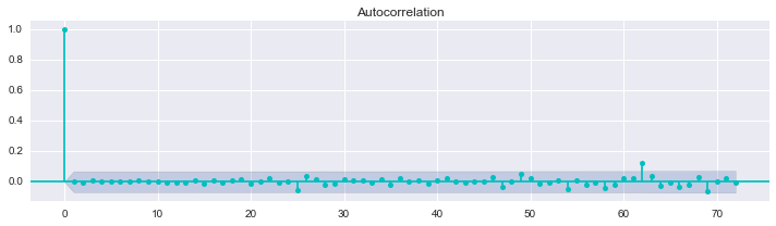
从下图也可以明显地看出以上结论。
fig, ax = plt.subplots(1, 1, figsize=(10, 3))
smg.tsa.plot_acf(result.resid, lags=72, ax=ax,color='c')
fig.tight_layout()
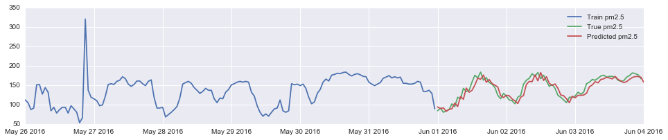
预测
对比6月初四天的预测情况,从曲线上看拟合的效果的非常理想,与实际值非常的吻合。
pm_train = pm[pm.index.month == 5]
pm_true = pm[pm.index.month == 6]
plt.figure(figsize = (16, 3))
plt.plot(pm_train.index.values[-144:], pm_train.avg[-144:], label = 'Train pm2.5')
plt.plot(pm_true.index.values[:72], pm_true.values[:72], label = 'True pm2.5')
plt.plot(pd.date_range("2016-06-01", "2016-06-04", freq="H").values,
         result.predict("2016-06-01", "2016-06-04"), label="Predicted pm2.5",)
plt.legend(loc='best')
plt.show()