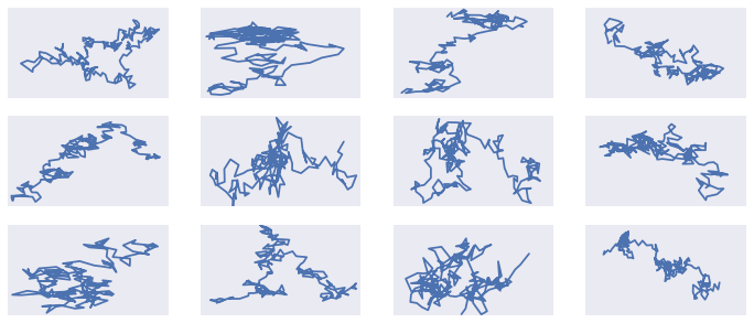
1. 随机漫步

%matplotlib inline
import numpy as np
import matplotlib.pyplot as plt
import seaborn as sns
from ipywidgets import *
from scipy.stats import norm

sns.set_style("darkgrid") #利用seaborn的style更漂亮一些
def random_walk(m,n,N=200):
    fig = plt.figure(figsize=(12,5))
    for i in range(1,m*n+1):
        r = np.random.randint(1,3,N)
        theta = np.radians(np.random.randint(0,361,N))
        x = np.cumsum(r*np.cos(theta))
        y = np.cumsum(r*np.sin(theta))
        plt.subplot(m,n,i) #切换到特定的subplot
        plt.plot(x,y)
        plt.xticks([]), plt.yticks([]) # 去掉ticks
    plt.show()

random_walk(3,4)

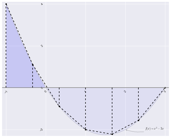
2. 画一二次函数及梯形法积分时的各个梯形

def f(x):
    return x*x - 3*x

a,b = -1,3
x = np.linspace(a,b,100,endpoint=True)
# 基本绘图
plt.figure(figsize=(10,8))
plt.plot(x,f(x),color='black',alpha=.1)

# 填充积分区域fill_between
plt.axhline(0,color='gray')
plt.fill_between(x,0,f(x),f(x)>0,color='blue',alpha=.15)
plt.fill_between(x,0,f(x),f(x)<0,color='blue',alpha=.05)

n = 7 #为凸显梯形和原来曲线的区别，把分割分数降低
# 画梯形
for i in range(n):
    x = np.linspace(a,b,n,endpoint=True)
    # 画垂直的线
    plt.plot([x[i],x[i]],[0,f(x[i])],color='black',linestyle='--')
    # 画特定的点
    plt.scatter(x[i],f(x[i]),20,color='black')
    if i==0: continue 
    # 画梯形最后的斜边
    plt.plot([x[i-1],x[i]],[f(x[i-1]),f(x[i])],color='black',linestyle='--')


ax = plt.gca()
# 注释
ax.annotate(r'$f(x)=x^2 - 3x$', xy=(2, -2), xytext=(2.5, -2),arrowprops=dict(arrowstyle="->", connectionstyle="arc3,rad=-.2"))

# 坐标轴平移
ax.spines['right'].set_color('none')
ax.spines['top'].set_color('none')
ax.spines['bottom'].set_position(('data',0))
ax.spines['left'].set_position(('data',0))

# 旋转label
for label in ax.get_xticklabels() + ax.get_yticklabels():
    label.set_rotation(45)

# 设置坐标轴的limit
plt.xlim([a-.1,b+.1]),plt.xticks([-1,0,1,2,3])
plt.ylim([-2.3,4.1]),plt.yticks([-2,0,2,4])
plt.show()

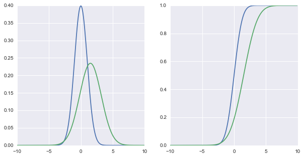
3. 交互函数

基本想法很简单，首先写一个你感兴趣的函数，然后指定想要交互参数就行。直接利用interact函数调用相应的函数，然后就会有交互效果，比如一个slider之类的。更多参考。

# 画一个正态分布曲线，调节其两个参数，看概率密度函数和累计分布函数
def f(mean,std):
    x = np.arange(-10, 10, 0.1)
    fig, axes = plt.subplots(1, 2, figsize=(10, 5))
    axes[0].plot(x,norm.pdf(x,0,1))
    axes[0].plot(x,norm.pdf(x,mean,std))
    axes[1].plot(x,norm.cdf(x,0,1))
    axes[1].plot(x,norm.cdf(x,mean,std)) 

#     fig, axes = plt.subplots(2, 2, figsize=(10, 5))
#     axes[0][0].plot(x,norm.pdf(x,0,1))
#     axes[0][1].plot(x,norm.cdf(x,0,1))
#     axes[1][0].plot(x,norm.pdf(x,mean,std))
#     axes[1][1].plot(x,norm.cdf(x,mean,std)) 

interact(f,mean=(-7.,7,0.5),std=(0.0,5));