随机优化

用常见的随机优化算法完成这周作业，包括随机搜索，爬山算法，随机开始爬山算法，模拟退火以及遗传算法。

import numpy as np
import scipy as sp
import scipy.optimize as opt
import matplotlib.pyplot as plt
%matplotlib inline

演示用函数

函数后面注释是最优理论解

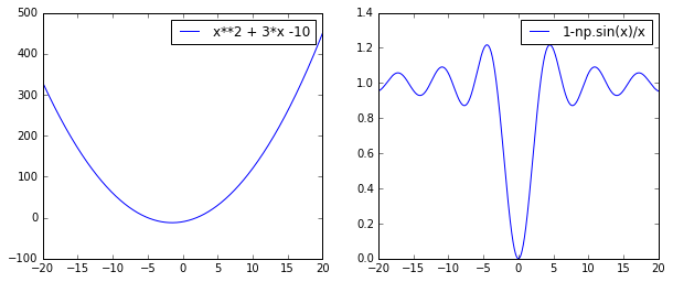
f = lambda x: x**2 + 3*x -10 # min at x = -1.5, y = -12.25
g = lambda x: 1-np.sin(x)/x # min at x = 0, y = 0

x = np.linspace(-20., 20., 1000)
y1, y2 = f(x), g(x)
fig, axes = plt.subplots(1,2,figsize=(10,4))
axes[0].plot(x,y1,label='x**2 + 3*x -10');axes[0].legend()
axes[1].plot(x,y2,label='1-np.sin(x)/x');axes[1].legend()
plt.show()

def demo_sol_plot(xguess,xmin):
    g = lambda x: 1-np.sin(x)/x
    x = np.linspace(-20., 20., 1000)
    y = g(x)
    plt.plot(x, y)
    plt.scatter(xguess, g(xguess), marker='o', s=100)
    plt.scatter(xmin, g(xmin), marker='v', s=100)
    plt.xlim(-20, 20);

随机搜索

简单粗暴，直接产生随机数代入，如果比之前更优，则保留，如果不是，则舍去。不是很靠谱的算法，但可以作为其他算法的baseline。给定区间，然后在此区间随机取值计算。

def random_search(f,a=0,b=1,n=1000):
    xmin = a
    ymin = f(xmin)
    x = (b - a) * np.random.random(n) + a
    for i in range(n):
        if f(x[i]) < ymin:
            xmin = x[i]
            ymin = f(xmin)

    return xmin

print random_search(f,-7,7,n=5000)
print random_search(g,-7,7,n=5000)

-1.49925162057
0.000193342497409

爬山算法

Hill climbing is a mathematical optimization technique which belongs to the family of local search. It is an iterative algorithm that starts with an arbitrary solution to a problem, then attempts to find a better solution by incrementally changing a single element of the solution. If the change produces a better solution, an incremental change is made to the new solution, repeating until no further improvements can be found.

爬山算法的名字很直接，很好理解。比如这里研究的函数，我们随机猜测一个值，然后以一定的步长移动，比如向左，如果更优，则继续往那一个方向移动，否则往相反的方向移动，直到迭代结束。爬山算法一个比较明显的缺点是容易陷入到局部最优。简单来说，爬山算法是向价值增长方向持续移动的循环过程。由于它的贪婪特性，使得在解决问题中容易得到局部极大值(Local maxima，指一个比所有邻居状态价值要高但是比全局最大值要低的状态)或者卡在高原区域(Plateaux，指一块连续且价值相等的区域)，对于前者，我们能采取随机重新开始(Random restart)以及模拟退火(Simulated annealing)的方法来改进，而对于后者的优化，侧向移动(Sideways move)则是一种不错的选择。

爬山算法与梯度下降法比较类似，一般更倾向于用梯度下降法(要求函数可导)，如果函数不可导，爬山算法是个很不错的选择。

这里是连续的函数求极值，其实用途远不止此，好多连续的问题，复杂度成指数级增长的问题，都有爬山算法的用武之地。

def hill_climbing(f,xmin,step=0.05,niter=10000):
    for i in range(niter):
        xl, xr = xmin - step, xmin + step
        if f(xl) < f(xmin):
            xmin = xl
            ymin = f(xmin)
            xl = xmin - step
        else:
            xmin = xr
            ymin = f(xmin)
            xr = xmin + step

    return xmin, ymin

hill_climbing(f,5)

(-1.4999999999999913, -12.25)

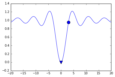
# 如果初始值给的好，结果比较理想
xmin, ymin = hill_climbing(g,3)
demo_sol_plot(3,xmin)

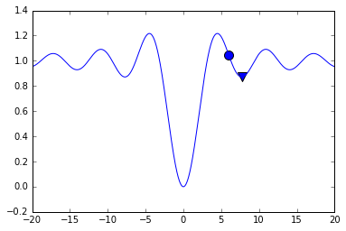
# 初始值给的不好，就会陷入局部最优
xmin, ymin = hill_climbing(g,6)
demo_sol_plot(6,xmin)

随机开始爬山算法

想法不能更粗暴了，如果一次爬山容易陷入局部最优，那就多随机爬几次，找到全局最优的几率还是蛮大的。从这个结果可以看出，得到全局最优的几率还是很不错的。

def random_restart_hill_climbing(f,a=-5,b=5,n_start=5,step=0.05,niter=10000):
    xs = np.random.random(n_start)*(b-a) + a # choose random number with in [a,b]
    x, y = [], []
    for i in range(n_start):
        xmin, ymin = hill_climbing(f,xs[i],step,niter)
        x.append(xmin)
        y.append(ymin)
    x,y = np.array(x), np.array(y)
    index = y.argmin()
    return x[index]

random_restart_hill_climbing(g,a=-5,b=5,n_start=6,step=0.05,niter=10000)

-0.0040896956486641128

遗传算法

遗传算法（Genetic Algorithm）是模拟达尔文生物进化论的自然选择和遗传学机理的生物进化过程的计算模型，是一种通过模拟自然进化过程搜索最优解的方法。遗传算法是从代表问题可能潜在的解集的一个种群（population）开始的，而一个种群则由经过基因（gene）编码的一定数目的个体(individual)组成。每个个体实际上是染色体(chromosome)带有特征的实体。染色体作为遗传物质的主要载体，即多个基因的集合，其内部表现（即基因型）是某种基因组合，它决定了个体的形状的外部表现，如黑头发的特征是由染色体中控制这一特征的某种基因组合决定的。因此，在一开始需要实现从表现型到基因型的映射即编码工作。由于仿照基因编码的工作很复杂，我们往往进行简化，如二进制编码，初代种群产生之后，按照适者生存和优胜劣汰的原理，逐代（generation）演化产生出越来越好的近似解，在每一代，根据问题域中个体的适应度（fitness）大小选择（selection）个体，并借助于自然遗传学的遗传算子（genetic operators）进行组合交叉（crossover）和变异（mutation），产生出代表新的解集的种群。这个过程将导致种群像自然进化一样的后生代种群比前代更加适应于环境，末代种群中的最优个体经过解码（decoding），可以作为问题近似最优解。

具体步骤如下：

• 初始化：设置进化代数计数器t=0，设置最大进化代数T，随机生成M个个体作为初始群体P(0)。
• 个体评价：计算群体P(t)中各个个体的适应度。
• 选择运算:将选择算子作用于群体。选择的目的是把优化的个体直接遗传到下一代或通过配对交叉产生新的个体再遗传到下一代。选择操作是建立在群体中个体的适应度评估基础上的。
• 交叉运算：将交叉算子作用于群体。遗传算法中起核心作用的就是交叉算子。
• 变异运算：将变异算子作用于群体。即是对群体中的个体串的某些基因座上的基因值作变动。群体P(t)经过选择、交叉、变异运算之后得到下一代群体P(t+1)。
• 终止条件判断:若t=T,则以进化过程中所得到的具有最大适应度个体作为最优解输出，终止计算。

1. 编码设计

遗传算法不能直接处理问题空间的参数，必须把它们转换成遗传空间的由基因按一定结构组成的染色体或个体。这一转换操作就叫做编码，也可以称作(问题的)表示(representation)。二进制编码是目前遗传算法中最常用的编码方法。即是由二进制字符集{0,1}产生通常的0,1字符串来表示问题空间的候选解。

我们建立十进制与二进制的映射，这样我们就能用基因序列表示数了，离我们的优化更近一步。二进制更像基因，便于crossover与mutation等操作。代码：

# map binary to decimal
def b2d(binary):
    shift = 0
    if a < 0:
        shift = abs(a)
        a, b = a + shift, b + shift
    t = 0
    for i in range(len(binary)):
        t = t + binary[i]*np.power(2,i)

    t = float(t*(b-a))/(np.power(2,gene_len)-1) # replace with gene len later
    return t - shift

2. 初始种群

遗传算法是对群体进行的进化操作，需要给其淮备一些表示起始搜索点的初始群体数据。

def generate_pop(pop_size,gene_len):
    pop = []
    for i in range(pop_size):
        individual = np.random.randint(2,size=gene_len)
        pop.append(individual)
    return np.array(pop)

3. 计算目标函数值

根据自变量与基因的转化关系式，求出每个个体的基因对应的自变量，然后将自变量代入函数f(x)，求出每个个体的目标函数值，我们是以此作为基础计算适应度的。

def get_obj_value(pop):
    '''
    Pass in population
    Decode population
    Evaluate it using function which interests us
    '''
    obj_value = []
    for i in range(len(pop)):
        x = b2d(pop[i]) # decode
        y = g(x) # evaluate
        obj_value.append(y)
    return np.array(obj_value)

4. 计算适应度

进化论中的适应度，是表示某一个体对环境的适应能力，也表示该个体繁殖后代的能力。遗传算法的适应度函数也叫评价函数，是用来判断群体中的个体的优劣程度的指标，它是根据所求问题的目标函数来进行评估的。

遗传算法在搜索进化过程中一般不需要其他外部信息，仅用评估函数来评估个体或解的优劣，并作为以后遗传操作的依据。由于遗传算法中，适应度函数要比较排序并在此基础上计算选择概率，所以适应度函数的值要取正值。由此可见，在不少场合，将目标函数映射成求最大值形式且函数值非负的适应度函数是必要的。

适应度函数的设计主要满足以下条件：

• 单值、连续、非负、最大化
• 合理、一致性

这里是求函数最小值，所以函数值越大，适应度越小。根据适应度的限制，可以基于函数值作如下构造：如果种群函数值均大于0，则直接用函数值reverse作为适应度；如果最小值小于0，则平移为正数，然后用最大值减去函数值，或直接reverse，代码如下：

def get_fitness(obj_value):
    '''
    Pass in obj_value of population
    Evaluate its fitness(Non-negative,single-valued,continous)
    Shift it necessary
    Target min. So the min obj_value gets highest fitness
    '''
    obj_min = np.min(obj_value)
    shift = 0 # ensure non negative
    if obj_min < 0:
        shift = np.abs(obj_min)
        obj_value = obj_value + shift
    # reverse it, bigger value, smaller fitness
    fitness = np.max(obj_value) - obj_value
    return np.array(fitness)

5. 自然选择

自然选择不必废话，这里的实现就是适应的高的，被选中的次数会多，这样优秀的个体基因会被更多地保留，具体实现使用轮盘赌算法。其具体步骤：

假设种群中共5个个体，fitness = [1,3,0,2,4] ，total_fitness = 10 ， fitness，值的大小表示在圆盘上的面积。在转动轮盘的过程中，单个模块的面积越大则被选中的概率越大。选择的方法是将fitness转化为[1,4,4,6,10], fitness/total_fitness = [0.1,0.4,0.4,0.6,1.0]。然后产生5个0-1之间的随机数，将随机数从小到大排序，假如是[0.05,0.2,0.7,0.8,0.9]，则将0号个体、1号个体、4号个体、4号个体、4号个体拷贝到新种群中。自然选择的结果使种群更符合条件了。

def selection(pop,fitness):
    '''
    Roulette wheel selection
    Individuals with greater fitness get select more times
    Pointers used to indicated the interval random number located
    '''
    total_fitness = np.sum(fitness)
    new_fitness = fitness/total_fitness # sum to 1
    new_fitness = np.cumsum(new_fitness) # cumsum it
    # generate random number between 0-1 and sort it
    prob = np.random.random(len(pop))
    prob = np.sort(prob)
    new_pop = pop
    pointer1, pointer2 = 0, 0
    # loop through prob list to select lucky individuals
    while pointer2 < len(pop):
        if prob[pointer2] < new_fitness[pointer1]:
            new_pop[pointer2] = pop[pointer1]
            pointer2 += 1
        else:
            pointer1 += 1
    return np.array(new_pop)

6. 交叉繁殖

交叉运算是遗传算法中产生新个体的主要操作过程，它以某一概率相互交换某两个个体之间的部分染色体。这里采用单点交叉的方法，其具体操作过程是：

• 先对群体进行随机配对；
• 其次随机设置交叉点位置；
• 最后再相互交换配对染色体之间的部分基因。

设个体a、b的基因是：

a = [1, 0, 0, 0, 0, 1, 1, 1, 0, 0]
b = [0, 0, 0, 1, 1, 0, 1, 1, 1, 1]
这两个个体发生基因交换的概率pc = 0.6.如果要发生基因交换，则产生一个随机数point表示基因交换的位置，假设point = 4,则：

a = [1, 0, 0, 0, 0, 1, 1, 1, 0, 0]
b = [0, 0, 0, 1, 1, 0, 1, 1, 1, 1]

交换后为：
a = [1, 0, 0, 0, 1, 0, 1, 1, 1, 1]
b = [0, 0, 0, 1, 0, 1, 1, 1, 0, 0]

def crossover(pop,pc=0.6):
    '''
    If random number < crossover prob, then pick a random point to cross
    '''
    for i in range(len(pop)-1):
        if np.random.random() < pc:
            cpoint = np.random.randint(0,len(pop[0])) # cross point
            temp1, temp2 = [], []
            temp1.extend(pop[i][0:cpoint])
            temp1.extend(pop[i+1][cpoint:len(pop[i])])
            temp2.extend(pop[i+1][0:cpoint])
            temp2.extend(pop[i][cpoint:len(pop[i])])
            pop[i] = temp1
            pop[i+1] = temp2
    return np.array(pop)

7. 变异

变异运算是对个体的某一个或某一些基因座上的基因值按某一较小的概率进行改变，它也是产生新个体的一种操作方法。这里采用基本位变异的方法来进行变异运算，其具体操作过程是：

• 首先确定出各个个体的基因变异位置
• 然后依照某一概率将变异点的原有基因值取反。

def mutation(pop,pm=0.001):
    '''
    If random number < pm, pick a random point, change it
    '''
    for i in range(len(pop)):
        if np.random.random() < pm:
            mpoint = np.random.randint(0,len(pop[i]))
            if pop[i][mpoint] == 1:
                pop[i][mpoint] = 0
            else:
                pop[i][mpoint] = 1
    return pop

8. 辅助函数

比如保留每一代里最优秀的个体，挑选出优秀个体群最有效的个体等。

def get_best(pop,fitness):
    '''
    Get individual with greatest fitness.
    '''
    best_index = np.array(fitness).argmax()
    best_individual = pop[best_index]
    return best_individual

def pick_result(f,results):
    result = results[0]
    for i in range(len(results)):
        if f(results[i]) < f(result):
            result = results[i]
    return result

9. 整合遗传算法

把上述函数封装到genetic_algo里，实现简单的遗传算法。从结果看，效果还行。

def genetic_algo(fun,a=-5,b=5,pop_size=50,gene_len=10,pc=0.5,pm=0.01,niter=25):
    '''
    f: Function within interval [a,b]
    pop_size: Population size
    gene_len: Gene length, choose it base on a,b
    pc: Crossover prob
    pm: Mutation prob
    '''
    import numpy as np
    def _generate_pop(pop_size,gene_len):
        pop = []
        for i in range(pop_size):
            individual = np.random.randint(2,size=gene_len)
            pop.append(individual)
        return np.array(pop)

    def _b2d(binary,a=a,b=b):
        '''Map binary to decimal'''
        shift = 0
        if a < 0:
            shift = abs(a)
            a, b = a + shift, b + shift
        t = 0
        for i in range(len(binary)):
            t = t + binary[i]*np.power(2,i)

        t = float(t*(b-a))/(np.power(2,gene_len)-1) # replace with gene len later
        return t - shift

    def _get_obj_value(pop):
        '''
        Pass in population; Decode population
        Evaluate it using function which interests us
        '''
        obj_value = []
        for i in range(len(pop)):
            x = _b2d(pop[i]) # decode
            y = fun(x) # evaluate
            obj_value.append(y)
        return np.array(obj_value)

    def _get_fitness(obj_value):
        '''
        Pass in obj_value of population
        Evaluate its fitness(Non-negative,single-valued,continous)
        Shift it necessary
        Target min. So the min obj_value gets highest fitness
        '''
        obj_min = np.min(obj_value)
        shift = 0 # ensure non negative
        if obj_min < 0:
            shift = np.abs(obj_min)
            obj_value = obj_value + shift
        # reverse it, bigger value, smaller fitness
        fitness = np.max(obj_value) - obj_value
        return np.array(fitness)

    def _selection(pop,fitness):
        '''
        Roulette wheel selection
        Individuals with greater fitness get select more times
        Pointers used to indicated the interval random number located
        '''
        total_fitness = np.sum(fitness)
        new_fitness = fitness/total_fitness # sum to 1
        new_fitness = np.cumsum(new_fitness) # cumsum it
        # generate random number between 0-1 and sort it
        prob = np.random.random(len(pop))
        prob = np.sort(prob)
        new_pop = pop
        pointer1, pointer2 = 0, 0
        # loop through prob list to select lucky individuals
        while pointer2 < len(pop):
            if prob[pointer2] < new_fitness[pointer1]:
                new_pop[pointer2] = pop[pointer1]
                pointer2 += 1
            else:
                pointer1 += 1
        return np.array(new_pop)

    def _crossover(pop,pc=pc):
        '''
        If random number < crossover prob, then pick a random point to cross
        '''
        for i in range(len(pop)-1):
            if np.random.random() < pc:
                cpoint = np.random.randint(0,len(pop[0])) # cross point
                temp1, temp2 = [], []
                temp1.extend(pop[i][0:cpoint])
                temp1.extend(pop[i+1][cpoint:len(pop[i])])
                temp2.extend(pop[i+1][0:cpoint])
                temp2.extend(pop[i][cpoint:len(pop[i])])
                pop[i] = temp1
                pop[i+1] = temp2
        return np.array(pop)

    def _mutation(pop,pm=pm):
        '''
        If random number < pm, pick a random point, change it
        '''
        for i in range(len(pop)):
            if np.random.random() < pm:
                mpoint = np.random.randint(0,len(pop[i]))
                if pop[i][mpoint] == 1:
                    pop[i][mpoint] = 0
                else:
                    pop[i][mpoint] = 1
        return pop

    def _get_best(pop,fitness):
        '''Get individual with greatest fitness in each generation'''
        best_index = np.array(fitness).argmax()
        best_individual = pop[best_index]
        return best_individual

    def _pick_result(fun,results):
        result = results[0]
        for i in range(len(results)):
            if fun(results[i]) < fun(result):
                result = results[i]
        return result

    pop = _generate_pop(pop_size,gene_len)
    results = []
    for i in range(niter):
        obj_value = _get_obj_value(pop)
        fitness = _get_fitness(obj_value)
        best = _get_best(pop,fitness)
        results.append(_b2d(best))
        pop = _selection(pop,fitness)
        pop = _crossover(pop,pc)
        pop = _mutation(pop,pm)

    return _pick_result(fun,results)

print genetic_algo(f,a=-5,b=5,pop_size=10000,niter=25)
print genetic_algo(g,a=-5,b=5,pop_size=10000,niter=25)

-1.50048875855
-0.00488758553275

模拟退火算法

模拟退火算法 (Simulated Annealing，SA) 最早的思想是由 N. Metropolis 等人于1953年提出。1983年, S. Kirkpatrick 等成功地将退火思想引入到组合优化领域。它是基于 Monte-Carlo 迭代求解策略的一种随机寻优算法，其出发点是基于物理中固体物质的退火过程与一般组合优化问题之间的相似性。模拟退火算法从某一较高初温出发，伴随温度参数的不断下降,结合概率突跳特性在解空间中随机寻找目标函数的全局最优解，即在局部最优解能概率性地跳出并最终趋于全局最优。

更多介绍参加各种百科. 这里算法实现后不是很稳定，还需要进一步搞明白哪里的问题。

def simulated_annealing(f,x_start,a=0,b=1,n=30):
    # n => number of cycles
    m = 50 # number of trails per cycle
    na = 0.0 # number of accept solutions
    p1 = 0.7 # probability of accepting worse solution at the start
    p50 = 0.001 # probability of accepting worse solution at the end

    # initial temperature
    t1 = -1.0/np.log(p1)
    # final temperature
    t50 = -1.0/np.log(p50)
    # fractional reduction every cycle
    frac = (t50/t1)**(1.0/(n-1.0))

    # initialize x
    x = np.zeros(n+1)
    x[0] = x_start
    xi = x_start
    na = na + 1

    # current best result so far
    xc = x[0]
    fc = f(xi)
    fs = np.zeros(n+1)
    fs[0] = fc

    # current temperature
    t = t1
    # DeltaE average
    DeltaE_avg = 0.0
    for i in range(n):
        # print 'Cycle: ' + str(i) + ' with Temperature: ' + str(t)
        for j in range(m):
            # new trails of points
            xi = xc + (np.random.random()-0.5)*(b-a)
            # Clip to upper and lower bounds
            xi = max(min(xi,b),a)
            DeltaE = abs(f(xi) - fc)
            if f(xi)>fc:
                # Initialize DeltaE_avg if a worse solution was found
                #   on the first iteration
                if (i==0 and j==0): DeltaE_avg = DeltaE
                # objective function is worse
                # generate probability of acceptance
                p = np.exp(-DeltaE/(DeltaE_avg * t))
                if np.random.random()<p:
                    # accept the worse solution
                    accept = True
                else:
                    accept = False
            else:
                # objective function is lower, automatically accept
                accept = True

            if accept:
                # update currently accepted solution
                xc = xi
                fc = f(xc)
                # increment number of accepted solutions
                na = na + 1.0
                # update DeltaE_avg
                DeltaE_avg = (DeltaE_avg * (na-1.0) +  DeltaE)/na

        # record the best x values at the end of every cycle
        x[i+1] = xc
        fs[i+1] = fc
        #lower the temperature for next cycle
        t = frac*t
    # return best solution, best objective and accepted sol and obj
    return xc,fc,x,fs

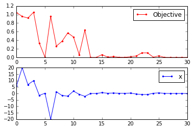
xc,fc,x,fs = simulated_annealing(g,6,-20,20)
xc # 理论解为0

0.0014153727555674678

迭代情况

从下图可以看到解的迭代情况，最后收敛到我们期望的值。

fig = plt.figure()
ax1 = fig.add_subplot(211)
ax1.plot(fs,'r.-')
ax1.legend(['Objective'])
ax2 = fig.add_subplot(212)
ax2.plot(x,'b.-')
ax2.legend(['x'])
plt.show()