概率密度函数估计

对上述收益率数据，使用参数方法和非参数方法估计其概率密度函数。参数方法选择正态分布和对数正态分布两种假设。基于上述三种方法分别计算收益率小于0的概率。

# 数据统计信息
info = stats.describe(rs)
info

DescribeResult(nobs=336, minmax=(-0.033330981281467977, 0.054449171819962665), mean=0.0003282497540976614, variance=0.00012068806084068744, skewness=0.3046124438496171, kurtosis=2.290568699302592)

正态分布

K-S检验是否符合正态分布：

单样本假设检验问题，可以采用K-S检验（ Kolmogorov-Smirnov test）。单样本K-S检验的原假设是给定的数据来自和原假设分布相同的分布，在SciPy中提供了kstest函数，参数分别是数据、拟检验的分布名称和对应的参数：

close.head(3)

Date
2013-01-04    2276.99
2013-01-07    2285.36
2013-01-08    2276.07
Name: Close, dtype: float64

# kstest使用练习
a = stats.norm.rvs(size=1000)
stat_val, p_val = stats.kstest(a, 'norm', (a.mean(), a.std()))
print 'KS-statistic D = %6.3f p-value = %6.4f' % (stat_val, p_val)

KS-statistic D =  0.020 p-value = 0.8195

mu = rs.mean()
sigma = rs.std()
stat_val, p_val = stats.kstest(rs, 'norm', (mu, sigma))
print 'KS-statistic D = %6.3f p-value = %6.4f' % (stat_val, p_val)

KS-statistic D =  0.066 p-value = 0.0988

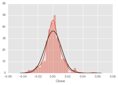
sns.distplot(rs,fit=stats.norm,kde=True);

T检验

P值大于0.05，所以在显著性水平为0.05的情况下，不能拒绝原假设，可能是正态分布，但信心不大，分布明明非常符合，但不知道为什么p值这么小。这里先接受原假设，即该数据通过了正态性的检验。在正态性的前提下，我们可进一步检验这组数据的均值是不是0。典型的方法是t检验（t-test），在scipy.stats单样本的t检验函数为ttest_1samp：

We can use the t-test to test whether the mean of our sample differs in a statistically significant way from the theoretical expectation

ttest_1samp() : Calculates the T-test for the mean of ONE group of scores.

例子：

from scipy import stats
np.random.seed(7654567)  # fix seed to get the same result
rvs = stats.norm.rvs(loc=5, scale=10, size=(50,2))
# Test if mean of random sample is equal to true mean, and different mean.
# We reject the null hypothesis in the second case and don't reject it in the first case.
stats.ttest_1samp(rvs,5.0)
# Out[0] (array([-0.68014479, -0.04323899]), array([ 0.49961383,  0.96568674]))
stats.ttest_1samp(rvs,0.0)
# Out[1] (array([ 2.77025808,  4.11038784]), array([ 0.00789095,  0.00014999]))

stat_val, p_val = stats.ttest_1samp(rs, 0)
print 'One-sample t-statistic D = %s, p-value = %s' % (stat_val, p_val)

One-sample t-statistic D = 0.547698931236, p-value = 0.584263368989

在给定显著性水平0.05的前提下，不能拒绝原假设：数据的均值为0。

极大似然估计：

之后可以调用fit函数来得到对应分布参数的极大似然估计（MLE, maximum-likelihood estimation）。以下代码示例了假设数据服从正态分布，用极大似然估计分布参数stats.norm.fit：
例子：

# Return MLEs for shape, location, and scale parameters from data
from scipy.stats import beta
a, b = 1., 2.
x = beta.rvs(a, b, size=1000)
# Now we can fit all four parameters (``a``, ``b``, ``loc`` and ``scale``):
a1, b1, loc1, scale1 = beta.fit(x)
# We can also use some prior knowledge about the dataset: let's keep ``loc`` and ``scale`` fixed:
a1, b1, loc1, scale1 = beta.fit(x, floc=0, fscale=1)

Note:

This fit is computed by maximizing a log-likelihood function, with penalty applied for samples outside of range of the distribution. The returned answer is not guaranteed to be the globally optimal MLE, it may only be locally optimal, or the optimization may fail altogether.

mu,sigma = rs.mean(), rs.std()
mu_mle, sigma_mle = stats.norm.fit(rs)

print "MLE data mean: %s VS %s Actual data mean" % (mu_mle,mu)
print "MLE data std: %s VS %s Actual data std" % (sigma_mle,sigma)

MLE data mean: 0.000328249754098 VS 0.000328249754098 Actual data mean
MLE data std: 0.0109694516811 VS 0.0109858117971 Actual data std

由于正态分布的最大似然估计非常常见，也可以推出参数的公式，所以这里用numpy函数计算然后和stats.norm.fit对比。结果参见此公式。可以看到与直接调用函数的结果吻合。

mu_1 = np.sum(rs)/len(rs)
sigma_1 = np.sqrt(np.sum((rs - mu_1)**2)/len(rs))
mu_1, sigma_1

(0.0003282497540976614, 0.010969451681074287)

收益率小于0的概率

norm_fit = stats.norm(loc=mu_mle,scale=sigma_mle)
norm_fit.cdf(0) # 均值在0附近，小于0的概率也应该在0.5附近

0.488063836882768

对数正态分布

题目有遗留的一个小错误，对数正态分布在这里不适用，当做了解了。
Wiki。
http://www.itl.nist.gov/div898/handbook/eda/section3/eda3669.htm

在概率论与统计学中，对数正态分布是对数为正态分布的任意随机变量的概率分布。如果 X 是服从正态分布的随机变量，则 exp(X) 服从对数正态分布；同样，如果 Y 服从对数正态分布，则 ln(Y) 服从正态分布。如果一个变量可以看作是许多很小独立因子的乘积，则这个变量可以看作是对数正态分布。一个典型的例子是股票投资的长期收益率，它可以看作是每天收益率的乘积。

A random variable which is log-normally distributed takes only positive real values.

python 里的stats.lognorm搞得好乱，一些参考：

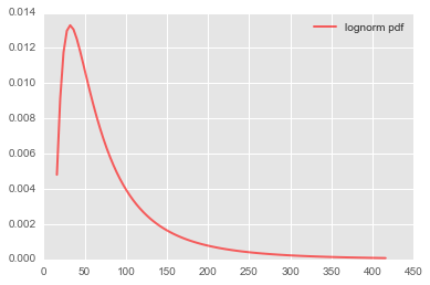
# **lognorm长啥样:**
import matplotlib.pyplot as plt
fig, ax = plt.subplots(1, 1)
# 三个参数的意义
s = 0.9; loc=10; scale=50
rv = stats.lognorm(s,loc,scale)
x = np.linspace(rv.ppf(0.01),rv.ppf(0.99), 100)
ax.plot(x, rv.pdf(x),'r-', lw=2, alpha=0.6, label='lognorm pdf')
plt.legend();

金融领域，一般股票价格趋向于对数正态分布，收益趋向于正态分布。看看收盘价直方图趋势：

# sns.distplot(close)
plt.hist(close,bins=20);

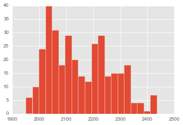
s, loc, scale = stats.lognorm.fit(close)
s, loc, scale
# stats.lognorm.fit(close) # return shape, loc and scale

(4.197772318507381, 1950.0099998853848, 5.1569526740479557)

参数估计