import numpy as np
from sklearn import datasets
数据集iris
iris = datasets.load_iris()
This data is stored in the .data member, which is a (n_samples, n_features) array.
type(iris) # Dictionary-like object that exposes its keys as attributes.
sklearn.datasets.base.Bunch
iris.keys()
['target_names', 'data', 'target', 'DESCR', 'feature_names']
iris.data.shape
(150, 4)
iris.feature_names # 列名
['sepal length (cm)',
 'sepal width (cm)',
 'petal length (cm)',
 'petal width (cm)']
The class of each observation is stored in the .target attribute of the dataset. This is an integer 1D array of length n_samples:
iris.target_names # 分类
array(['setosa', 'versicolor', 'virginica'],
      dtype='|S10')
iris.target.shape
(150,)
np.unique(iris.target)
array([0, 1, 2])
学习与预测
In scikit-learn, we learn from existing data by creating an estimator and calling its fit(X, Y) method
from sklearn import svm
clf = svm.LinearSVC() # Linear Support Vector Classification.
type(clf)
sklearn.svm.classes.LinearSVC
clf.fit(iris.data, iris.target) #Fit the model according to the given training data
LinearSVC(C=1.0, class_weight=None, dual=True, fit_intercept=True,
     intercept_scaling=1, loss='squared_hinge', max_iter=1000,
     multi_class='ovr', penalty='l2', random_state=None, tol=0.0001,
     verbose=0)
Once we have learned from the data, we can use our model to predict the most likely outcome on unseen data:
clf.predict([[5.0, 3.6, 1.3, 0.25]]) # 属于setosa
array([0])
Access attributes
clf.classes_
array([0, 1, 2])
print clf.coef_
[[ 0.18424051  0.45122844 -0.8079464  -0.45071164]
 [ 0.05178528 -0.89052546  0.404389   -0.93791474]
 [-0.8507913  -0.98669598  1.38090215  1.86552929]]
分类
KNN
The simplest possible classifier is the nearest neighbor: given a new observation, take the label of the training samples closest to it in n-dimensional space, where n is the number of features in each sample.
from sklearn import neighbors
knn = neighbors.KNeighborsClassifier()
knn.fit(iris.data, iris.target)
KNeighborsClassifier(algorithm='auto', leaf_size=30, metric='minkowski',
           metric_params=None, n_jobs=1, n_neighbors=5, p=2,
           weights='uniform')
knn.predict([[0.1, 0.2, 0.3, 0.4]])
array([0])
Training set and testing set
When experimenting with learning algorithms, it is important not to test the prediction of an estimator on the data used to fit the estimator. Indeed, with the kNN estimator, we would always get perfect prediction on the training set.
# get random order
perm = np.random.permutation(iris.target.size) # int or array like
iris.data = iris.data[perm]
iris.target = iris.target[perm]
knn.fit(iris.data[:100], iris.target[:100])
KNeighborsClassifier(algorithm='auto', leaf_size=30, metric='minkowski',
           metric_params=None, n_jobs=1, n_neighbors=5, p=2,
           weights='uniform')
# score
knn.score(iris.data[100:], iris.target[100:])
0.95999999999999996
SVM for classification
SVMs try to construct a hyperplane maximizing the margin between the two classes. It selects a subset of the input, called the support vectors, which are the observations closest to the separating hyperplane.
from sklearn import svm
svc = svm.SVC(kernel='linear')
svc.fit(iris.data, iris.target)
SVC(C=1.0, cache_size=200, class_weight=None, coef0=0.0,
  decision_function_shape=None, degree=3, gamma='auto', kernel='linear',
  max_iter=-1, probability=False, random_state=None, shrinking=True,
  tol=0.001, verbose=False)
Play with digits data
digits = datasets.load_digits()
digits.keys()
['images', 'data', 'target_names', 'DESCR', 'target']
print digits.images.shape
print digits.data.shape # transformed from images 8*8 data
print digits.target_names
(1797, 8, 8)
(1797, 64)
[0 1 2 3 4 5 6 7 8 9]
digits.images[0]
array([[  0.,   0.,   5.,  13.,   9.,   1.,   0.,   0.],
       [  0.,   0.,  13.,  15.,  10.,  15.,   5.,   0.],
       [  0.,   3.,  15.,   2.,   0.,  11.,   8.,   0.],
       [  0.,   4.,  12.,   0.,   0.,   8.,   8.,   0.],
       [  0.,   5.,   8.,   0.,   0.,   9.,   8.,   0.],
       [  0.,   4.,  11.,   0.,   1.,  12.,   7.,   0.],
       [  0.,   2.,  14.,   5.,  10.,  12.,   0.,   0.],
       [  0.,   0.,   6.,  13.,  10.,   0.,   0.,   0.]])
digits.data[0]
array([  0.,   0.,   5.,  13.,   9.,   1.,   0.,   0.,   0.,   0.,  13.,
        15.,  10.,  15.,   5.,   0.,   0.,   3.,  15.,   2.,   0.,  11.,
         8.,   0.,   0.,   4.,  12.,   0.,   0.,   8.,   8.,   0.,   0.,
         5.,   8.,   0.,   0.,   9.,   8.,   0.,   0.,   4.,  11.,   0.,
         1.,  12.,   7.,   0.,   0.,   2.,  14.,   5.,  10.,  12.,   0.,
         0.,   0.,   0.,   6.,  13.,  10.,   0.,   0.,   0.])
digits.target[3]
3
Digits datasets SVM learn
Classes are not always separable by a hyperplane, so it would be desirable to have a decision function that is not linear but that may be for instance polynomial or exponential:
对比linear, ploy and rbf,对digits数据,poly的效果最好,rbf最差。
i = int(0.85*len(digits.target))
for kernel in ['linear', 'poly', 'rbf']:
    svc = svm.SVC(kernel= kernel)
    svc.fit(digits.data[:i],digits.target[:i])
    print kernel + ': ' + str(svc.score(digits.data[i:], digits.target[i:]))
linear: 0.925925925926
poly: 0.940740740741
rbf: 0.42962962963
Clustering
Given the iris dataset, if we knew that there were 3 types of iris, but did not have access to their labels, we could try unsupervised learning: we could cluster the observations into several groups by some criterion
K-means clustering
The simplest clustering algorithm is k-means. This divides a set into k clusters, assigning each observation to a cluster so as to minimize the distance of that observation (in n-dimensional space) to the cluster’s mean; the means are then recomputed. This operation is run iteratively until the clusters converge, for a maximum for max_iter rounds
from sklearn import cluster
k_means = cluster.KMeans(n_clusters=3)
k_means.fit(iris.data)
KMeans(copy_x=True, init='k-means++', max_iter=300, n_clusters=3, n_init=10,
    n_jobs=1, precompute_distances='auto', random_state=None, tol=0.0001,
    verbose=0)
print k_means.labels_[::10]
print iris.target[::10]
[2 0 1 0 2 1 0 1 0 0 1 2 2 0 1]
[2 1 0 2 2 0 1 0 1 1 0 2 2 1 0]
Application to Image Compression
Clustering can be seen as a way of choosing a small number of information from the observations (like a projection on a smaller space). For instance, this can be used to posterize an image (conversion of a continuous gradation of tone to several regions of fewer tones):
from scipy import misc
face = misc.face(gray=True).astype(np.float32) # np.array
print face.shape
print face.reshape((-1,1)).shape
(768, 1024)
(786432, 1)
X = face.reshape((-1,1)) # We need an (n_sample, n_feature) array
K = k_means = cluster.KMeans(n_clusters=5)
k_means.fit(X)
KMeans(copy_x=True, init='k-means++', max_iter=300, n_clusters=5, n_init=10,
    n_jobs=1, precompute_distances='auto', random_state=None, tol=0.0001,
    verbose=0)
values = k_means.cluster_centers_.squeeze()
labels = k_means.labels_
face_compressed = np.choose(labels,values)
face_compressed.shape = face.shape
fig, axes = plt.subplots(1,2,figsize=(12,8))
axes[0].imshow(face)
axes[1].imshow(face_compressed)
plt.show()

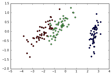
Dimension Reduction with PCA

The cloud of points spanned by the observations above is very flat in one direction, so that one feature can almost be exactly computed using the 2 other. PCA finds the directions in which the data is not flat and it can reduce the dimensionality of the data by projecting on a subspace.
from sklearn import decomposition
pca = decomposition.PCA(n_components=2)
pca.fit(iris.data)
X = pca.transform(iris.data)
iris.data.shape
(150, 4)
X.shape
(150, 2)
plt.scatter(X[:,0],X[:,1],c=iris.target);
PCA is not just useful for visualization of high dimensional datasets. It can also be used as a preprocessing step to help speed up supervised methods that are not efficient with high dimensions.
Linear model
Diabetes dataset
The diabetes dataset consists of 10 physiological variables (age, sex, weight, blood pressure) measure on 442 patients, and an indication of disease progression after one year:
diabetes = datasets.load_diabetes()
diabetes_X_train = diabetes.data[:-20]
diabetes_X_test = diabetes.data[-20:]
diabetes_Y_train = diabetes.target[:-20]
diabetes_Y_test = diabetes.target[-20:]
The task at hand is to predict disease prediction from physiological variables.
Sparse model
diabetes.data.shape
(442, 10)
有十个维度,去掉信息含量低的特征。
To improve the conditioning of the problem (uninformative variables, mitigate the curse of dimensionality, as a feature selection preprocessing, etc.), it would be interesting to select only the informative features and set non-informative ones to 0. This penalization approach, called Lasso, can set some coefficients to zero. Such methods are called sparse method, and sparsity can be seen as an application of Occam’s razor: prefer simpler models to complex ones.
from sklearn import linear_model
regr = linear_model.Lasso(alpha=.3)
regr.fit(diabetes_X_train,diabetes_Y_train)
Lasso(alpha=0.3, copy_X=True, fit_intercept=True, max_iter=1000,
   normalize=False, positive=False, precompute=False, random_state=None,
   selection='cyclic', tol=0.0001, warm_start=False)
regr.coef_ # 系数很稀疏
array([   0.        ,   -0.        ,  497.34075682,  199.17441034,
         -0.        ,   -0.        , -118.89291545,    0.        ,
        430.9379595 ,    0.        ])
regr.score(diabetes_X_test,diabetes_Y_test)
0.55108354530029779
与linear regression对比
lin = linear_model.LinearRegression()
lin.fit(diabetes_X_train,diabetes_Y_train)
/usr/local/lib/python2.7/site-packages/scipy/linalg/basic.py:884: RuntimeWarning: internal gelsd driver lwork query error, required iwork dimension not returned. This is likely the result of LAPACK bug 0038, fixed in LAPACK 3.2.2 (released July 21, 2010). Falling back to 'gelss' driver.
  warnings.warn(mesg, RuntimeWarning)


LinearRegression(copy_X=True, fit_intercept=True, n_jobs=1, normalize=False)
lin.score(diabetes_X_test,diabetes_Y_test)
0.58507530226905724
Cross validated estimators
Get parameter
Cross-validation to set a parameter can be done more efficiently on an algorithm-by-algorithm basis. This is why, for certain estimators, the scikit-learn exposes “CV” estimators, that set their parameter automatically by cross-validation:
These estimators are called similarly to their counterparts, with ‘CV’ appended to their name.
lasso = linear_model.LassoCV()
X_diabetes = diabetes.data
Y_diabetes = diabetes.target
lasso.fit(X_diabetes,Y_diabetes)
LassoCV(alphas=None, copy_X=True, cv=None, eps=0.001, fit_intercept=True,
    max_iter=1000, n_alphas=100, n_jobs=1, normalize=False, positive=False,
    precompute='auto', random_state=None, selection='cyclic', tol=0.0001,
    verbose=False)
lasso.alpha_
0.012291895087486173
Find the best alpha
la = linear_model.LassoCV()
la.fit(diabetes_X_train,diabetes_Y_train)
la.alpha_
0.034628679642636641
# 得分最高
regr_alpha = linear_model.Lasso(alpha=la.alpha_)
regr_alpha.fit(diabetes_X_train,diabetes_Y_train)
regr_alpha.score(diabetes_X_test,diabetes_Y_test)
0.58835979803792404