导入模块
from scipy import stats
from scipy.stats import norm
import matplotlib.pyplot as plt
import numpy as np
%matplotlib inline
import seaborn as sns
sns.set(style="whitegrid")
分布
There are two general distribution classes that have been implemented for encapsulating continuous random variables and discrete random variables.
常见方法
连续型分布常见方法
- rvs: Random Variates
- pdf: Probability Density Function
- cdf: Cumulative Distribution Function
- sf: Survival Function (1-CDF)
- ppf: Percent Point Function (Inverse of CDF)
- isf: Inverse Survival Function (Inverse of SF)
- stats: Return mean, variance, (Fisher’s) skew, or (Fisher’s) kurtosis
- moment: non-central moments of the distribution
cdf
norm.cdf(0) # Cumulative Distribution Function
0.5
norm.cdf([-1., 0, 1])
array([ 0.15865525, 0.5 , 0.84134475])
mean, std, var ..
norm.mean(), norm.std(), norm.var()
(0.0, 1.0, 1.0)
ppf
To find the median of a distribution we can use the percent point function ppf, which is the inverse of the cdf:
norm.ppf(0.5) #中位数为零
0.0
rvs
从分布中产生随机变量
norm.rvs(size=5)
array([ 0.39589009, 1.77897676, -0.2289895 , 2.09622412, -1.53182512])
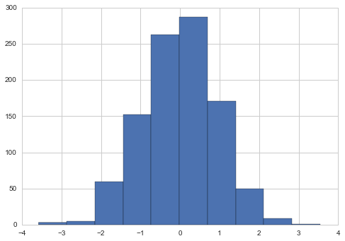
a = norm.rvs(size=1000)
plt.hist(a)
plt.show()
seed
Note that drawing random numbers relies on generators from numpy.random package. In the example above, the specific stream of random numbers is not reproducible across runs. To achieve reproducibility, you can explicitly seed a global variable.
np.random.seed(1234)
norm.rvs(size=5, random_state=1234) # 每次运行结果一样
array([ 0.47143516, -1.19097569, 1.43270697, -0.3126519 , -0.72058873])
shifting and scaling
All continuous distributions take loc and scale as keyword parameters to adjust the location and scale of the distribution, e.g. for the standard normal distribution the location is the mean and the scale is the standard deviation.
norm
# no shift or scale
norm.stats()
(array(0.0), array(1.0))
norm(1,1).stats()
(array(1.0), array(1.0))
norm.stats(loc=1,scale=1)
(array(1.0), array(1.0))
def pair_plot(a,b):
    fig = plt.figure(figsize=(8,4))
    ax1,ax2 = fig.add_subplot(121), fig.add_subplot(122)
    ax1.hist(a);ax2.hist(b)
    plt.show()
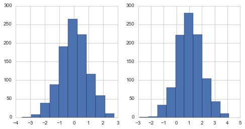
a = norm.rvs(size=1000)
b = norm(loc=1,scale=1).rvs(size=1000)
pair_plot(a,b)
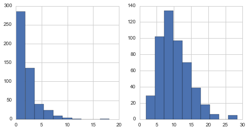
expon
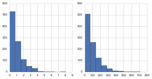
from scipy.stats import expon
a = expon.rvs(size=1000)
b = expon(scale=100).rvs(size=1000)
pair_plot(a,b)
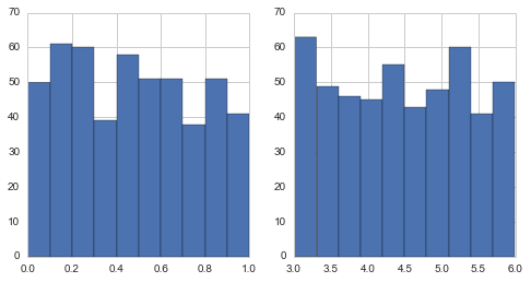
uniform
from scipy.stats import uniform
# This distribution is constant between `loc` and ``loc + scale``.
uniform.cdf([0,0.5,0.7])
array([ 0. , 0.5, 0.7])
uniform.cdf([0, 1, 2, 3, 4, 5], loc = 1, scale = 4)
array([ 0. , 0. , 0.25, 0.5 , 0.75, 1. ])
a = uniform.rvs(size=500)
b = uniform.rvs(loc=3,scale=3,size=500)
pair_plot(a,b)
shape parameters
While a general continuous random variable can be shifted and scaled with the loc and scale parameters, some distributions require additional shape parameters. For instance, the gamma distribution
from scipy.stats import gamma
# gamma.rvs(a, loc=0, scale=1, size=1, random_state=None)
gamma(1, scale=2.).stats()
(array(2.0), array(4.0))
gamma(3, scale=2.).stats()
(array(6.0), array(12.0))
a = gamma(1,scale=2.).rvs(size=500)
b = gamma(a=5,scale=2.).rvs(size=500)
pair_plot(a,b)
Freezing a Distribution
assing the loc and scale keywords time and again can become quite bothersome. The concept of freezing a RV is used to solve such problems.
rv = norm(loc=2,scale=1)
rv.mean()
2.0
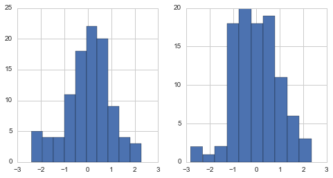
一个T分布例子
T分布。
np.random.seed(282629734)
x = stats.t.rvs(10, size=1000) # n=10
a = stats.t(10).rvs(size=100)
b = stats.t(50).rvs(size=100)
pair_plot(a,b)
基本统计量
x[0:5]
array([-0.20862765, -1.29471404, -1.63750825, -1.40201994, -0.97847465])
print x.max(), x.min() # equivalent to np.max(x), np.min(x)
5.26327732981 -3.78975572422
print x.mean(), x.var() # equivalent to np.mean(x), np.var(x)
0.0140610663985 1.28899386208
理论值对比
理论值
# stats.t.stats: some statistics of the given RV
# moments: composed of letters ['mvsk'] defining which moments to compute
# 对应mean, var skew kurtosis
m, v, s, k = stats.t.stats(10, moments='mvsk')
stats.t.stats(10,moments='mvsk')
(array(0.0), array(1.25), array(0.0), array(1.0))
实际值
# Computes several descriptive statistics of the passed array.
# 对应size,minmax,sample mean...
n, (smin, smax), sm, sv, ss, sk = stats.describe(x)
stats.describe(x)
DescribeResult(nobs=1000, minmax=(-3.7897557242248197, 5.2632773298071651), mean=0.014061066398468425, variance=1.2902841462255106, skewness=0.21652778283120952, kurtosis=1.055594041706331)
对比
print m, sm # sampe mean
0.0 0.0140610663985
print v, sv
1.25 1.29028414623
print s, ss
0.0 0.216527782831
print k, sk
1.0 1.05559404171
注意:
stats.describe uses the unbiased estimator for the variance, while np.var is the biased estimator
T检验
We can use the t-test to test whether the mean of our sample differs in a statistically significant way from the theoretical expectation
ttest_1samp(): Calculates the T-test for the mean of ONE group of scores.
例子:
from scipy import stats
np.random.seed(7654567)  # fix seed to get the same result
rvs = stats.norm.rvs(loc=5, scale=10, size=(50,2))
# Test if mean of random sample is equal to true mean, and different mean.
# We reject the null hypothesis in the second case and don't reject it in the first case.
stats.ttest_1samp(rvs,5.0)
# Out[0] (array([-0.68014479, -0.04323899]), array([ 0.49961383,  0.96568674]))
stats.ttest_1samp(rvs,0.0)
# Out[1] (array([ 2.77025808,  4.11038784]), array([ 0.00789095,  0.00014999]))
print 't-statistic = %6.3f pvalue = %6.4f' % stats.ttest_1samp(x, m)
t-statistic = 0.391 pvalue = 0.6955
手动实现
tt = (sm-m)/np.sqrt(sv/float(n))  # t-statistic for mean
pval = stats.t.sf(np.abs(tt), n-1)*2  # two-sided pvalue = Prob(abs(t)>tt)
print 't-statistic = %6.3f pvalue = %6.4f' % (tt, pval)
t-statistic = 0.391 pvalue = 0.6955
K-S检验
In statistics, the Kolmogorov–Smirnov test (K–S test or KS test) is a nonparametric test of the equality of continuous, one-dimensional probability distributions that can be used to compare a sample with a reference probability distribution (one-sample K–S test), or to compare two samples (two-sample K–S test). The Kolmogorov–Smirnov statistic quantifies a distance between the empirical distribution function of the sample and the cumulative distribution function of the reference distribution, or between the empirical distribution functions of two samples. The null distribution of this statistic is calculated under the null hypothesis that the sample is drawn from the reference distribution (in the one-sample case) or that the samples are drawn from the same distribution (in the two-sample case). In each case, the distributions considered under the null hypothesis are continuous distributions but are otherwise unrestricted.
The two-sample K–S test is one of the most useful and general nonparametric methods for comparing two samples, as it is sensitive to differences in both location and shape of the empirical cumulative distribution functions of the two samples.
kstest in scipy.stats
This performs a test of the distribution G(x) of an observed random variable against a given distribution F(x). Under the null hypothesis the two distributions are identical, G(x)=F(x).
例子
from scipy import stats
x = np.linspace(-15, 15, 9)
stats.kstest(x, 'norm')
# Out[0] (0.44435602715924361, 0.038850142705171065)
# The Kolmogorov-Smirnov test can be used to test the hypothesis that the sample comes from the standard t-distribution
print 'KS-statistic D = %6.3f pvalue = %6.4f' % stats.kstest(x, 't', (10,))
KS-statistic D = 0.016 pvalue = 0.9606
In real applications, we don’t know what the underlying distribution is. If we perform the Kolmogorov-Smirnov test of our sample against the standard normal distribution, then we also cannot reject the hypothesis that our sample was generated by the normal distribution given that in this example the p-value is almost 40%.
print 'KS-statistic D = %6.3f pvalue = %6.4f' % stats.kstest(x,'norm')
KS-statistic D = 0.028 pvalue = 0.3949
Tails of the distribution
cdf, ppf, sf, isf等方法。
We can check the upper tail of the distribution. We can use the percent point function ppf, which is the inverse of the cdf function, to obtain the critical values, or, more directly, we can use the inverse of the survival function(sf: Survival function (1 -
cdf) at x of the given RV) (isf: Inverse survival function (inverse ofsf) at q of the given RV).
crit01, crit05, crit10 = stats.t.ppf([1-0.01, 1-0.05, 1-0.10], 10)
print 'critical values from ppf at 1%%, 5%% and 10%% %8.4f %8.4f %8.4f'% (crit01, crit05, crit10)
critical values from ppf at 1%, 5% and 10% 2.7638 1.8125 1.3722
# tuple
print 'critical values from isf at 1%%, 5%% and 10%% %8.4f %8.4f %8.4f'% tuple(stats.t.isf([0.01,0.05,0.10],10))
critical values from isf at 1%, 5% and 10% 2.7638 1.8125 1.3722
Comparing two samples
In the following, we are given two samples, which can come either from the same or from different distribution, and we want to test whether these samples have the same statistical properties.
ttest_ind(rvs1,rvs2)
# with same mean
rvs1 = stats.norm.rvs(loc=5, scale=10, size=500)
rvs2 = stats.norm.rvs(loc=5, scale=10, size=500)
stats.ttest_ind(rvs1, rvs2)
Ttest_indResult(statistic=-0.51425157176625691, pvalue=0.60718996593022279)
# with different value
rvs3 = stats.norm.rvs(loc=8, scale=10, size=500)
stats.ttest_ind(rvs1, rvs3)
Ttest_indResult(statistic=-4.6192600501294256, pvalue=4.3544947395228574e-06)
Kolmogorov-Smirnov test for two samples ks_2samp
# same mean
stats.ks_2samp(rvs1, rvs2)
Ks_2sampResult(statistic=0.040000000000000036, pvalue=0.81104101838088782)
# different mean
stats.ks_2samp(rvs1, rvs3)
Ks_2sampResult(statistic=0.15600000000000003, pvalue=8.5374993202435991e-06)
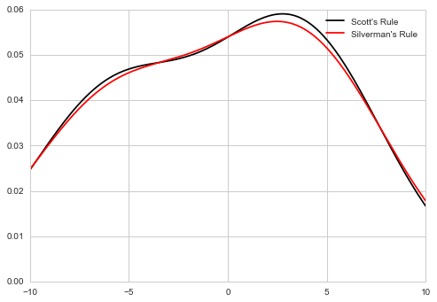
Kernel Density Estimation
A common task in statistics is to estimate the probability density function (PDF) of a random variable from a set of data samples. This task is called density estimation. The most well-known tool to do this is the histogram. A histogram is a useful tool for visualization (mainly because everyone understands it), but doesn’t use the available data very efficiently. Kernel density estimation (KDE) is a more efficient tool for the same task. The gaussian_kde estimator can be used to estimate the PDF of univariate as well as multivariate data. It works best if the data is unimodal.
x1 = np.array([-7, -5, 1, 4, 5], dtype=np.float)
kde1 = stats.gaussian_kde(x1)
kde2 = stats.gaussian_kde(x1, bw_method='silverman')
fig = plt.figure()
ax = fig.add_subplot(111)
ax.plot(x1, np.zeros(x1.shape), 'b+', ms=20)  # rug plot
x_eval = np.linspace(-10, 10, num=200)
ax.plot(x_eval, kde1(x_eval), 'k-', label="Scott's Rule")
ax.plot(x_eval, kde2(x_eval), 'r-', label="Silverman's Rule")
plt.legend()
plt.show()
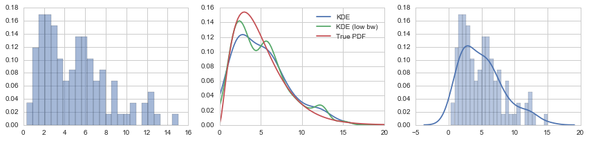
np.random.seed(0)
X = stats.chi2(df=5)
X_samples = X.rvs(100)
kde = stats.kde.gaussian_kde(X_samples)
kde_low_bw = stats.kde.gaussian_kde(X_samples, bw_method=0.25)
x = np.linspace(0, 20, 100)
fig, axes = plt.subplots(1, 3, figsize=(12, 3))

axes[0].hist(X_samples, normed=True, alpha=0.5, bins=25)
axes[1].plot(x, kde(x), label="KDE")
axes[1].plot(x, kde_low_bw(x), label="KDE (low bw)")
axes[1].plot(x, X.pdf(x), label="True PDF")
axes[1].legend()
sns.distplot(X_samples, bins=25, ax=axes[2])

fig.tight_layout()
kde.resample(10)
array([[ 1.75376869,  0.5812183 ,  8.19080268,  1.38539326,  7.56980335,
         1.16144715,  3.07747215,  5.69498716,  1.25685068,  9.55169736]])
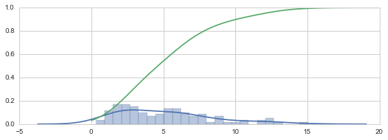
def _kde_cdf(x):
    return kde.integrate_box_1d(-np.inf, x)
kde_cdf = np.vectorize(_kde_cdf)
fig, ax = plt.subplots(1, 1, figsize=(8, 3))

sns.distplot(X_samples, bins=25, ax=ax)
x = np.linspace(0, 20, 100)
ax.plot(x, kde_cdf(x))

fig.tight_layout()