作业
- 写一个函数,能将一个多类别变量转化为多个二元虚拟变量,不能用sklearn库
- 写一个函数,实现交叉验证功能,不能用sklearn库
- 使用sklearn库的其他分类方法,来预测titanic的生存情况
- 研究kaggle中的Digit Recognizer数据,尝试用一些特征工程来提取数字特征,并放入分类器中观察预测准确率,相对直接使用原始变量是否有提升
- 用NumPy库实现K-nearest neighbors回归或分类
- 用NumPy库实现gradient descent算法,用以计算线性回归或岭回归系数
- 用NumPy库实现gradient ascent算法,用以计算logistic回归的回归系数。
import numpy as np
import pandas as pd
from sklearn import cross_validation
import seaborn as sns
import matplotlib.pyplot as plt
%matplotlib inline
sns.set_style()
多类别变量转化为二元虚拟变量
写一个函数,能将一个多类别变量转化为多个二元虚拟变量,不能用sklearn库。
随机产生多类别变量数据
cat = list('abc')
lst = []
for i in range(100):
    index = np.random.randint(0,3)
    lst.append(cat[index])
df = pd.DataFrame({'category' : lst})
df.head(3)
| category | |
|---|---|
| 0 | b |
| 1 | b |
| 2 | c |
Pandas的get_dummies函数
pd.get_dummies, Convert categorical variable into dummy/indicator variables.可以看到,如果对应的值为b,则转换为[0.0, 1.0, 0.0];若果对应的值为c,则转换为[0.0,0.0,1.0].
pd.get_dummies(df).head()
| category_a | category_b | category_c | |
|---|---|---|---|
| 0 | 0.0 | 1.0 | 0.0 |
| 1 | 0.0 | 1.0 | 0.0 |
| 2 | 0.0 | 0.0 | 1.0 |
| 3 | 0.0 | 0.0 | 1.0 |
| 4 | 0.0 | 1.0 | 0.0 |
定义函数
函数很简单,取给定列的unique值,就是所有的类别,然后对给定列所有的值map一下就可以。
def my_dummy(df,column):
    """
    Input a dataframe with category column and convert categorical variable into dummy/indicator variables
    """
    cats = df[column].unique()
    cats.sort()
    for cat in cats:
        new_col = column + '_' + cat
        df[new_col] = df[column].map(lambda x: 1. if x==cat else 0.)
    return df
df = my_dummy(df,'category')
df.head()
| category | category_a | category_b | category_c | |
|---|---|---|---|---|
| 0 | b | 0.0 | 1.0 | 0.0 |
| 1 | b | 0.0 | 1.0 | 0.0 |
| 2 | c | 0.0 | 0.0 | 1.0 |
| 3 | c | 0.0 | 0.0 | 1.0 |
| 4 | b | 0.0 | 1.0 | 0.0 |
KNN算法
用NumPy库实现K-nearest neighbors回归或分类。

邻近算法,或者说K最近邻(kNN,k-NearestNeighbor)分类算法是数据挖掘分类技术中最简单的方法之一。所谓K最近邻,就是k个最近的邻居的意思,说的是每个样本都可以用它最接近的k个邻居来代表。
kNN算法的核心思想是如果一个样本在特征空间中的k个最相邻的样本中的大多数属于某一个类别,则该样本也属于这个类别,并具有这个类别上样本的特性。该方法在确定分类决策上只依据最邻近的一个或者几个样本的类别来决定待分样本所属的类别。 kNN方法在类别决策时,只与极少量的相邻样本有关。由于kNN方法主要靠周围有限的邻近的样本,而不是靠判别类域的方法来确定所属类别的,因此对于类域的交叉或重叠较多的待分样本集来说,kNN方法较其他方法更为适合。
简单的理解,我有一组数据,比如每个数据都是n维向量,那么我们可以在n维空间表示这个数据,这些数据都有对应的标签值,也就是我们感兴趣的预测变量。那么当我们接到一个新的数据的时候,我们可以计算这个新数据和我们已知的训练数据之间的距离,找出其中最近的k个数据,对这k个数据对应的标签值取平均值就是我们得出的预测值。简单粗暴,谁离我近,就认为谁能代表我,我就用你们的属性作为我的属性。具体的简单代码实现如下。
1. 数据
这里例子来自《集体智慧编程》给的葡萄酒的价格模型。葡萄酒的价格假设由酒的等级与储藏年代共同决定,给定rating与age之后,就能给出酒的价格。
def wineprice(rating,age):
    """
    Input rating & age of wine and Output it's price.
    Example:
    ------
    input = [80.,20.] ===> output = 140.0
    """
    peak_age = rating - 50 # year before peak year will be more expensive
    price = rating/2.
    if age > peak_age:
        price = price*(5 -(age-peak_age))
    else:
        price = price*(5*((age+1)/peak_age))

    if price < 0: price=0
    return price
a = wineprice(80.,20.)
a
140.0
根据上述的价格模型,我们产生n=500瓶酒及价格,同时为价格随机加减了20%来体现随机性,同时增加预测的难度。注意基本数据都是numpy里的ndarray,为了便于向量化计算,同时又有强大的broadcast功能,计算首选。
def wineset(n=500):
    """
    Input wineset size n and return feature array and target array.
    Example:
    ------
    n = 3
    X = np.array([[80,20],[95,30],[100,15]])
    y = np.array([140.0,163.6,80.0])
    """
    X,y  = [], []
    for i in range(n):
        rating = np.random.random()*50 + 50
        age = np.random.random()*50
        # get reference price
        price = wineprice(rating,age)
        # add some noise
        price = price*(np.random.random()*0.4 + 0.8) #[0.8,1.2]
        X.append([rating,age])
        y.append(price)
    return np.array(X), np.array(y)
X,y = wineset(500)
X[:3]
array([[ 88.89511317,  11.63751282],
       [ 91.57171713,  39.76279923],
       [ 98.38870877,  14.07015414]])
2. 相似度:欧氏距离
knn的名字叫K近邻,如何叫“近”,我们需要一个数学上的定义,最常见的是用欧式距离,二维三维的时候对应平面或空间距离。
算法实现里需要的是给定一个新的数据,需要计算其与训练数据组之间所有点之间的距离,注意是不同的维度,给定的新数据只是一个sample,而训练数据是n组,n个sample,计算的时候需要注意,不过numpy可以自动broadcat,可以很好地take care of it。
def euclidean(arr1,arr2):
    """
    Input two array and output theie distance list.
    Example:
    ------
    arr1 = np.array([[3,20],[2,30],[2,15]])
    arr2 = np.array([[2,20],[2,20],[2,20]]) # broadcasted, np.array([2,20]) and [2,20] also work.
    d    = np.array([1,20,5])
    """
    ds = np.sum((arr1 - arr2)**2,axis=1)
    return np.sqrt(ds)
arr1 = np.array([[3,20],[2,30],[2,15]])
arr2 = np.array([[2,20],[2,20],[2,20]])
euclidean(arr1,arr2)
array([ 1., 10., 5.])
提供一个简洁的接口,给定训练数据X和新sample v,然后返回排序好的距离,以及对应的index(我们要以此索引近邻们对应的标签值)。
def getdistance(X,v):
    """
    Input train data set X and a sample, output the distance between each other with index.
    Example:
    ------
    X = np.array([[3,20],[2,30],[2,15]])
    v = np.array([2,20]) # to be broadcasted
    Output dlist = np.array([1,5,10]), index = np.array([0,2,1])
    """
    dlist = euclidean(X,np.array(v))
    index = np.argsort(dlist)
    dlist.sort()
    # dlist_with_index = np.stack((dlist,index),axis=1)
    return dlist, index
dlist, index = getdistance(X,[80.,20.])
3. KNN算法
knn算法具体实现的时候很简单,调用前面的函数,计算出排序好的距离列表,然后对其前k项对应的标签值取均值即可。可以用该knn算法与实际的价格模型对比,发现精度还不错。
def knn(X,y,v,kn=3):
    """
    Input train data and train target, output the average price of new sample.
    X = X_train; y = y_train
    k: number of neighbors
    """
    dlist, index = getdistance(X,v)
    avg = 0.0
    for i in range(kn):
        avg = avg + y[index[i]]
    avg = avg / kn
    return avg
knn(X,y,[95.0,5.0],kn=3)
32.043042600537092
wineprice(95.0,5.0)
31.666666666666664
4. 加权KNN
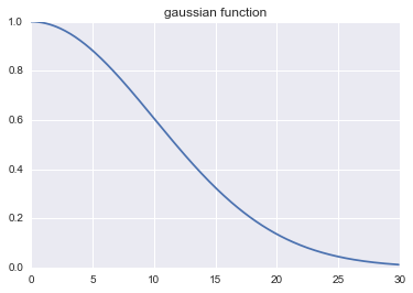
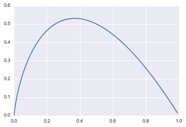
以上是KNN的基本算法,有一个问题就是该算法给所有的近邻分配相等的权重,这个还可以这样改进,就是给更近的邻居分配更大的权重(你离我更近,那我就认为你跟我更相似,就给你分配更大的权重),而较远的邻居的权重相应地减少,取其加权平均。需要一个能把距离转换为权重的函数,gaussian函数是一个比较普遍的选择,下图可以看到gaussian函数的衰减趋势。从下面的单例可以看出其效果要比knn算法的效果要好,不过只是单个例子,不具有说服力,后面给出更可信的评价。
def gaussian(dist,sigma=10.0):
    """Input a distance and return it's weight"""
    weight = np.exp(-dist**2/(2*sigma**2))
    return weight
x1 = np.arange(0,30,0.1)
y1 = gaussian(x1)
plt.title('gaussian function')
plt.plot(x1,y1);
def knn_weight(X,y,v,kn=3):
    dlist, index = getdistance(X,v)
    avg = 0.0
    total_weight = 0
    for i in range(kn):
        weight = gaussian(dlist[i])
        avg = avg + weight*y[index[i]]
        total_weight = total_weight + weight
    avg = avg/total_weight
    return avg
knn_weight(X,y,[95.0,5.0],kn=3)
32.063929602836012
交叉验证
写一个函数,实现交叉验证功能,不能用sklearn库。
交叉验证(Cross-Validation): 有时亦称循环估计, 是一种统计学上将数据样本切割成较小子集的实用方法。于是可以先在一个子集上做分析, 而其它子集则用来做后续对此分析的确认及验证。 一开始的子集被称为训练集。而其它的子集则被称为验证集或测试集。常见交叉验证方法如下:
Holdout Method(保留)
- 方法:将原始数据随机分为两组,一组做为训练集,一组做为验证集,利用训练集训练分类器,然后利用验证集验证模型,记录最后的分类准确率为此Hold-OutMethod下分类器的性能指标.。Holdout Method相对于K-fold Cross Validation 又称Double cross-validation ,或相对K-CV称 2-fold cross-validation(2-CV)
- 优点:好处的处理简单,只需随机把原始数据分为两组即可
- 缺点:严格意义来说Holdout Method并不能算是CV,因为这种方法没有达到交叉的思想,由于是随机的将原始数据分组,所以最后验证集分类准确率的高低与原始数据的分组有很大的关系,所以这种方法得到的结果其实并不具有说服性.(主要原因是 训练集样本数太少,通常不足以代表母体样本的分布,导致 test 阶段辨识率容易出现明显落差。此外,2-CV 中一分为二的分子集方法的变异度大,往往无法达到「实验过程必须可以被复制」的要求。)
K-fold Cross Validation(k折叠)
- 方法:作为Holdout Methon的演进,将原始数据分成K组(一般是均分),将每个子集数据分别做一次验证集,其余的K-1组子集数据作为训练集,这样会得到K个模型,用这K个模型最终的验证集的分类准确率的平均数作为此K-CV下分类器的性能指标.K一般大于等于2,实际操作时一般从3开始取,只有在原始数据集合数据量小的时候才会尝试取2. 而K-CV 的实验共需要建立 k 个models,并计算 k 次 test sets 的平均辨识率。在实作上,k 要够大才能使各回合中的 训练样本数够多,一般而言 k=10 (作为一个经验参数)算是相当足够了。
- 优点:K-CV可以有效的避免过学习以及欠学习状态的发生,最后得到的结果也比较具有说服性.
- 缺点:K值选取上
Leave-One-Out Cross Validation(留一)
- 方法:如果设原始数据有N个样本,那么留一就是N-CV,即每个样本单独作为验证集,其余的N-1个样本作为训练集,所以留一会得到N个模型,用这N个模型最终的验证集的分类准确率的平均数作为此下LOO-CV分类器的性能指标.
- 优点:相比于前面的K-CV,留一有两个明显的优点:
- a.每一回合中几乎所有的样本皆用于训练模型,因此最接近原始样本的分布,这样评估所得的结果比较可靠。
- b. 实验过程中没有随机因素会影响实验数据,确保实验过程是可以被复制的.
- 缺点:计算成本高,因为需要建立的模型数量与原始数据样本数量相同,当原始数据样本数量相当多时,LOO-CV在实作上便有困难几乎就是不显示,除非每次训练分类器得到模型的速度很快,或是可以用并行化计算减少计算所需的时间。
Holdout method方法的想法很简单,给一个train_size,然后算法就会在指定的比例(train_size)处把数据分为两部分,然后返回。
# Holdout method
def my_train_test_split(X,y,train_size=0.95,shuffle=True):
    """
    Input X,y, split them and out put X_train, X_test; y_train, y_test.
    Example:
    ------
    X = np.array([[0, 1],[2, 3],[4, 5],[6, 7],[8, 9]])
    y = np.array([0, 1, 2, 3, 4])
    Then
    X_train = np.array([[4, 5],[0, 1],[6, 7]])
    X_test = np.array([[2, 3],[8, 9]])
    y_train = np.array([2, 0, 3])
    y_test = np.array([1, 4])
    """
    order = np.arange(len(y))
    if shuffle:
        order = np.random.permutation(order)
    border = int(train_size*len(y))
    X_train, X_test = X[:border], X[border:]
    y_train, y_test = y[:border], y[border:]
    return X_train, X_test, y_train, y_test
K folds算法是把数据分成k份,进行k此循环,每次不同的份分别来充当测试组数据。但是注意,该算法不直接操作数据,而是产生一个迭代器,返回训练和测试数据的索引。看docstring里的例子应该很清楚。
# k folds 产生一个迭代器
def my_KFold(n,n_folds=5,shuffe=False):
    """
    K-Folds cross validation iterator.
    Provides train/test indices to split data in train test sets. Split dataset
    into k consecutive folds (without shuffling by default).
    Each fold is then used a validation set once while the k - 1 remaining fold form the training set.
    Example:
    ------
    X = np.array([[1, 2], [3, 4], [1, 2], [3, 4]])
    y = np.array([1, 2, 3, 4])
    kf = KFold(4, n_folds=2)
    for train_index, test_index in kf:
        X_train, X_test = X[train_index], X[test_index]
        y_train, y_test = y[train_index], y[test_index]
        print("TRAIN:", train_index, "TEST:", test_index)
    TRAIN: [2 3] TEST: [0 1]
    TRAIN: [0 1] TEST: [2 3]
    """
    idx = np.arange(n)
    if shuffe:
        idx = np.random.permutation(idx)
    fold_sizes = (n // n_folds) * np.ones(n_folds, dtype=np.int) # folds have size n // n_folds
    fold_sizes[:n % n_folds] += 1 # The first n % n_folds folds have size n // n_folds + 1
    current = 0
    for fold_size in fold_sizes:
        start, stop = current, current + fold_size
        train_index = list(np.concatenate((idx[:start], idx[stop:])))
        test_index = list(idx[start:stop])
        yield train_index, test_index
        current = stop # move one step forward
X1 = np.array([[1, 2], [3, 4], [1, 2], [3, 4]])
y1 = np.array([1, 2, 3, 4])
kf = my_KFold(4, n_folds=2)
for train_index, test_index in kf:
    X_train, X_test = X1[train_index], X1[test_index]
    y_train, y_test = y1[train_index], y1[test_index]
    print("TRAIN:", train_index, "TEST:", test_index)
('TRAIN:', [2, 3], 'TEST:', [0, 1])
('TRAIN:', [0, 1], 'TEST:', [2, 3])
KNN算法交叉验证
万事俱备只欠东风,已经实现了KNN算法以及交叉验证功能,我们就可以利用交叉验证的思想为我们的算法选择合适的参数,这也是交叉验证主要目标之一。
评价算法
首先我们用一个函数评价算法,给定训练数据与测试数据,计算平均的计算误差,这是评价算法好坏的重要指标。
def test_algo(alg,X_train,X_test,y_train,y_test,kn=3):
    error = 0.0
    for i in range(len(y_test)):
        guess = alg(X_train,y_train,X_test[i],kn=kn)
        error += (y_test[i] - guess)**2
    return error/len(y_test)
X_train,X_test,y_train,y_test = my_train_test_split(X,y,train_size=0.8)
test_algo(knn,X_train,X_test,y_train,y_test,kn=3)
783.80937472673656
交叉验证
得到平均误差,注意这里KFold 生成器的使用。
def my_cross_validate(alg,X,y,n_folds=100,kn=3):
    error = 0.0
    kf = my_KFold(len(y), n_folds=n_folds)
    for train_index, test_index in kf:
        X_train, X_test = X[train_index], X[test_index]
        y_train, y_test = y[train_index], y[test_index]
        error += test_algo(alg,X_train,X_test,y_train,y_test,kn=kn)
    return error/n_folds
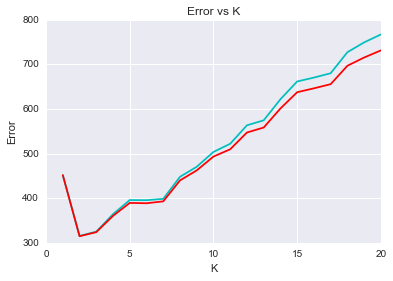
选最好的k值
从下图可以看出,模型表现随k值的变化呈现一个折现型,当为1时,表现较差;当取2,3的时候,模型表现还不错;但当k继续增加的时候,模型表现急剧下降。同时knn_weight算法要略优于knn算法,有一点点改进。
errors1, errors2 = [], []
for i in range(20):
    error1 = my_cross_validate(knn,X,y,kn=i+1)
    error2 = my_cross_validate(knn_weight,X,y,kn=i+1)
    errors1.append(error1)
    errors2.append(error2)
xs = np.arange(len(errors1)) + 1
plt.plot(xs,errors1,color='c')
plt.plot(xs,errors2,color='r')
plt.xlabel('K')
plt.ylabel('Error')
plt.title('Error vs K');
Kmeans聚类

K-means算法是很典型的基于距离的聚类算法,采用距离作为相似性的评价指标,即认为两个对象的距离越近,其相似度就越大。该算法认为簇是由距离靠近的对象组成的,因此把得到紧凑且独立的簇作为最终目标。动图来源.
k个初始类聚类中心点的选取对聚类结果具有较大的影响,因为在该算法第一步中是随机的选取任意k个对象作为初始聚类的中心,初始地代表一个簇。该算法在每次迭代中对数据集中剩余的每个对象,根据其与各个簇中心的距离将每个对象重新赋给最近的簇。当考察完所有数据对象后,一次迭代运算完成,新的聚类中心被计算出来。如果在一次迭代前后,J的值没有发生变化,说明算法已经收敛。
算法步骤:
- 创建k个点作为起始支点(随机选择)
- 当任意一个簇的分配结果发生改变的时候
- 对数据集的每个数据点
- 对每个质心
- 计算质心与数据点之间的距离
- 将数据分配到距离其最近的簇
- 对每个质心
- 对每一簇,计算簇中所有点的均值并将其均值作为质心
- 对数据集的每个数据点
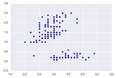
iris
我们用非常著名的iris数据集。
from sklearn import datasets
iris = datasets.load_iris()
X, y = iris.data, iris.target
data = X[:,[1,3]] # 为了便于可视化,只取两个维度
plt.scatter(data[:,0],data[:,1]);
欧式距离
计算欧式距离,我们需要为每个点找到离其最近的质心,需要用这个辅助函数。
def distance(p1,p2):
    """
    Return Eclud distance between two points.
    p1 = np.array([0,0]), p2 = np.array([1,1]) => 1.414
    """
    tmp = np.sum((p1-p2)**2)
    return np.sqrt(tmp)

distance(np.array([0,0]),np.array([1,1]))
1.4142135623730951
随机质心
在给定数据范围内随机产生k个簇心,作为初始的簇。随机数都在给定数据的范围之内dmin + (dmax - dmin) * np.random.rand(k)实现。
def rand_center(data,k):
    """Generate k center within the range of data set."""
    n = data.shape[1] # features
    centroids = np.zeros((k,n)) # init with (0,0)....
    for i in range(n):
        dmin, dmax = np.min(data[:,i]), np.max(data[:,i])
        centroids[:,i] = dmin + (dmax - dmin) * np.random.rand(k)
    return centroids

centroids = rand_center(data,2)
centroids
array([[ 2.15198267,  2.42476808],
       [ 2.77985426,  0.57839675]])
k均值聚类
- Once a set of centroids $\mu_k$ is available, the clusters are updated to contain the points closest in distance to each centroid.
- Given a set of clusters, the centroids are recalculated as the means of all points belonging to a cluster.
这个基本的算法只需要明白两点。
- 给定一组质心,则簇更新,所有的点被分配到离其最近的质心中。
- 给定k簇,则质心更新,所有的质心用其簇的均值替换
当簇不在有更新的时候,迭代停止。当然kmeans有个缺点,就是可能陷入局部最小值,有改进的方法,比如二分k均值,当然也可以多计算几次,去效果好的结果。
def kmeans(data,k=2):
    def _distance(p1,p2):
        """
        Return Eclud distance between two points.
        p1 = np.array([0,0]), p2 = np.array([1,1]) => 1.414
        """
        tmp = np.sum((p1-p2)**2)
        return np.sqrt(tmp)
    def _rand_center(data,k):
        """Generate k center within the range of data set."""
        n = data.shape[1] # features
        centroids = np.zeros((k,n)) # init with (0,0)....
        for i in range(n):
            dmin, dmax = np.min(data[:,i]), np.max(data[:,i])
            centroids[:,i] = dmin + (dmax - dmin) * np.random.rand(k)
        return centroids

    def _converged(centroids1, centroids2):

        # if centroids not changed, we say 'converged'
         set1 = set([tuple(c) for c in centroids1])
         set2 = set([tuple(c) for c in centroids2])
         return (set1 == set2)


    n = data.shape[0] # number of entries
    centroids = _rand_center(data,k)
    label = np.zeros(n,dtype=np.int) # track the nearest centroid
    assement = np.zeros(n) # for the assement of our model
    converged = False

    while not converged:
        old_centroids = centroids
        for i in range(n):
            # determine the nearest centroid and track it with label
            min_dist, min_index = np.inf, -1
            for j in range(k):
                dist = _distance(data[i],centroids[j])
                if dist < min_dist:
                    min_dist, min_index = dist, j
                    label[i] = j
            assement[i] = _distance(data[i],centroids[label[i]])**2

        # update centroid
        for m in range(k):
            centroids[m] = np.mean(data[label==m],axis=0)
        converged = _converged(old_centroids,centroids)
    return centroids, label, np.sum(assement)
由于算法可能局部收敛的问题,随机多运行几次,取最优值
best_assement = np.inf
best_centroids = None
best_label = None
for i in range(10):
centroids, label, assement = kmeans(data,2)
if assement < best_assement:
best_assement = assement
best_centroids = centroids
best_label = label
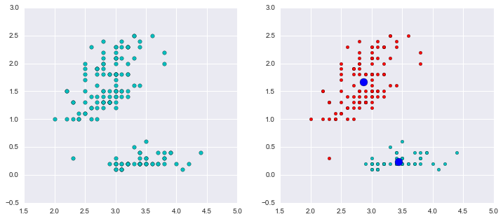
data0 = data[best_label==0]
data1 = data[best_label==1]
如下图,我们把数据分为两簇,绿色的点是每个簇的质心,从图示效果看,聚类效果还不错。
fig, (ax1,ax2) = plt.subplots(1,2,figsize=(12,5))
ax1.scatter(data[:,0],data[:,1],c='c',s=30,marker='o')
ax2.scatter(data0[:,0],data0[:,1],c='r')
ax2.scatter(data1[:,0],data1[:,1],c='c')
ax2.scatter(centroids[:,0],centroids[:,1],c='b',s=120,marker='o')
plt.show()
决策回归树
同样也来自《集体编程的智慧》一书的例子。以下数据分别表示来源网站,位置,是否阅读过FAQ,浏览网页数,选择服务类型。我们的目标就是根据前面的用户特征预测其可能选择的服务类型。
data = [['slashdot','USA','yes',18,'None'],
    ['google','France','yes',23,'Premium'],
    ['digg','USA','yes',24,'Basic'],
    ['kiwitobes','France','yes',23,'Basic'],
    ['google','UK','no',21,'Premium'],
    ['(direct)','New Zealand','no',12,'None'],
    ['(direct)','UK','no',21,'Basic'],
    ['google','USA','no',24,'Premium'],
    ['slashdot','France','yes',19,'None'],
    ['digg','USA','no',18,'None'],
    ['google','UK','no',18,'None'],
    ['kiwitobes','UK','no',19,'None'],
    ['digg','New Zealand','yes',12,'Basic'],
    ['google','UK','yes',18,'Basic'],
    ['kiwitobes','France','yes',19,'Basic']]
引入决策树
表达形式Node:
决策树用一系列节点表示,类似与二叉树,给出一个根节点,就能揪出下面所有的页节点。与二叉树的区别就是这里的节点存储了更多的信息,这里以性别(gender)为例(male, female).
- col:用以判断的列索引,比如gender位于数据矩阵的第2列,则self.col = 1
- value:匹配的目标值,如果是male,那么到这个节点,需要用gender的值与male对比,True就去true branch, False就去false branch
- tb和fb:类似于二叉树的左孩子和右孩子,这里是true branch和false branch
- results:当前分支的结果,是一个字典
class Node:
    def __init__(self,col=-1,value=None,results=None,tb=None,fb=None):
        self.col = col # col index to be tested
        self.value = value # to be matched for result to be true
        self.results = results
        self.tb = tb # true
        self.fb = fb # false
对决策树进行训练
根据一个判断条件,比如性别,把数据分为两组。
data[0]
['slashdot', 'USA', 'yes', 18, 'None']
def divide(rows, column,value):
    split_fun = None
    if type(value) in [int, float]:
        split_fun = lambda row: row[column] >= value # 如果value是数值型,则判断是否 >= value
    else:
        split_fun = lambda row: row[column] == value # 若果value不是,则判断是否 == value
    # split it
    set1 = [row for row in rows if split_fun(row)]
    set2 = [row for row in rows if not split_fun(row)]
    return (set1, set2)

divide(data,2,'yes')
([['slashdot', 'USA', 'yes', 18, 'None'],
  ['google', 'France', 'yes', 23, 'Premium'],
  ['digg', 'USA', 'yes', 24, 'Basic'],
  ['kiwitobes', 'France', 'yes', 23, 'Basic'],
  ['slashdot', 'France', 'yes', 19, 'None'],
  ['digg', 'New Zealand', 'yes', 12, 'Basic'],
  ['google', 'UK', 'yes', 18, 'Basic'],
  ['kiwitobes', 'France', 'yes', 19, 'Basic']],
 [['google', 'UK', 'no', 21, 'Premium'],
  ['(direct)', 'New Zealand', 'no', 12, 'None'],
  ['(direct)', 'UK', 'no', 21, 'Basic'],
  ['google', 'USA', 'no', 24, 'Premium'],
  ['digg', 'USA', 'no', 18, 'None'],
  ['google', 'UK', 'no', 18, 'None'],
  ['kiwitobes', 'UK', 'no', 19, 'None']])
熵
我们要选择好的决策方案,但好是如何衡量的呢?比较常见的是用基尼不纯度或者熵来表示,但之前我们需要一个函数来对一个集合中元素进行计数,从而评价其混乱程度。
def uni_val_counts(rows):
    results = {}
    for row in rows:
        r = row[len(row) - 1] # 结果默认在最后一列
        if r not in results:
            results[r] = 0
        results[r] += 1
    return results
def entropy(rows):
    # sum of -p(x)*log(p(x))
    from math import log
    log2 = lambda x: log(x) / log(2)
    results = uni_val_counts(rows)
    ent = 0.0
    for r in results.keys():
        p = float(results[r]) / len(rows)
        ent = ent - p*log2(p)
    return ent
# 熵的大致走势
x1 = np.arange(0.0001,1,0.01)
plt.plot(x1,-x1*np.log2(x1));
set1, set2 = divide(data,2,'yes')
print entropy(data)
print entropy(set1)
print entropy(set2)
1.52192809489
1.2987949407
1.37878349349
信息增益(information gain)
熵能衡量出一组数据的混乱程度,但不能判断一个属性的好坏,也就是数据被分组后有没有混乱程度有没有降低。这里需要引入信息增益,即当前的熵与两个新群组加权平均的熵之间的差值。如果信息增益最大,我们认为这个属性最好。当信息增益不大于零的时候,停止对分支的拆分。
pset1 = float(len(set1)) / len(data)
pset2 = float(len(set2)) / len(data)
gain = entropy(data) - pset1*entropy(set1) - pset2*entropy(set2)
print "Information gain %s" % gain
Information gain 0.18580516289
构造树
以递归的方式构造树。传入数据,算法会遍历(第一层循环)所有的feature列(col)(不包括要预测的target),然后对特定的列(如第i列),遍历(第二层循环)其中的unique值(value),从中选出最好的值。这样会得到best_criteria = (col, value),这样就选出最合适的标准。如果最好的标准有information gain,则继续递归,直到没有信息增益位置,返回。
如果有信息增益,则用true branch和false branch继续进行子树的构造。
如果没有信息增益,则返回节点,往上递归。
def build_tree(rows):
    if len(rows) == 0:
        return Node()
    current_score = entropy(rows)
    # keep track of best criteria
    best_gain = 0.0
    best_criteria = None
    best_sets = None

    column_count = len(rows[0]) - 1 # last column for target
    for col in range(0,column_count):
        column_values = {}
        for row in rows:
            column_values[row[col]] = 1 # get unique values in each col
        for value in column_values.keys():
            (set1, set2) = divide(rows,col,value) # split along col by value
            # information gain
            p = float(len(set1)) / len(rows)
            gain = current_score - p*entropy(set1) - (1-p)*entropy(set2)
            if gain > best_gain and len(set1) > 0 and len(set2) > 0:
                best_gain = gain
                best_criteria = (col, value)
                best_sets = (set1, set2)
        # build true branch and false branch
    if best_gain > 0:
        true_branch = build_tree(best_sets[0])
        false_branch = build_tree(best_sets[1])
        return Node(col=best_criteria[0],value=best_criteria[1],tb=true_branch,fb=false_branch)
    else:
        return Node(results=uni_val_counts(rows))

tree = build_tree(data)
显示树
def print_tree(tree,indent=''):
    if tree.results != None:
        print str(tree.results)
    else:
        print str(tree.col) + ':' + str(tree.value) + '? '
        print indent + 'T-->',
        print_tree(tree.tb,indent='  ')
        print indent + 'F-->',
        print_tree(tree.fb, indent='  ')

print_tree(tree)
3:21?
T--> 0:google?
  T--> {'Premium': 3}
  F--> {'Basic': 3}
F--> 2:yes?
  T--> 0:slashdot?
  T--> {'None': 2}
  F--> {'Basic': 3}
  F--> {'None': 4}
分类
def classify(observation,tree):
    if tree.results != None:
        return tree.results
    else:
        v = observation[tree.col]
        branch = None
        if type(v) in [int,float]:
            if v >= tree.value: branch = tree.tb
            else: branch = tree.fb
        else:
            if v == tree.value: branch = tree.tb
            else: branch = tree.fb
        return classify(observation,branch)

classify(['digg','USA','yes',24],tree)
{'Basic': 3}
Digit Reconizer
研究kaggle中的Digit Recognizer数据,尝试用一些特征工程来提取数字特征,并放入分类器中观察预测准确率,相对直接使用原始变量是否有提升
from sklearn.cross_validation import train_test_split
from sklearn import linear_model
from sklearn import tree
from sklearn import neighbors
from sklearn import ensemble
from sklearn import decomposition
from sklearn import metrics
digit = pd.read_csv('digit/train.csv')
digit.head(2)
| label | pixel0 | pixel1 | pixel2 | pixel3 | pixel4 | pixel5 | pixel6 | pixel7 | pixel8 | ... | pixel774 | pixel775 | pixel776 | pixel777 | pixel778 | pixel779 | pixel780 | pixel781 | pixel782 | pixel783 | |
|---|---|---|---|---|---|---|---|---|---|---|---|---|---|---|---|---|---|---|---|---|---|
| 0 | 1 | 0 | 0 | 0 | 0 | 0 | 0 | 0 | 0 | 0 | ... | 0 | 0 | 0 | 0 | 0 | 0 | 0 | 0 | 0 | 0 |
| 1 | 0 | 0 | 0 | 0 | 0 | 0 | 0 | 0 | 0 | 0 | ... | 0 | 0 | 0 | 0 | 0 | 0 | 0 | 0 | 0 | 0 |
2 rows × 785 columns
digit.info()
<class 'pandas.core.frame.DataFrame'>
RangeIndex: 42000 entries, 0 to 41999
Columns: 785 entries, label to pixel783
dtypes: int64(785)
memory usage: 251.5 MB
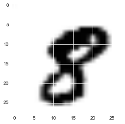
图形展现
数据代表的是各个像素的值,用plt.imshow()来展现其代表的图形。
d1 = digit.values[10]
pix = []
for i in range(28):
    pix.append([])
    for j in range(28):
        pix[i].append(d1[i*28+j])
plt.imshow(pix);
Slice数据
由于数据比较大,这里只slice其中一部分计算。
digit.columns = range(785);
X,y = digit[range(1,785)][:4000], digit[0][:4000] # only slice 4000 to speed up
降维
由于初始数据对应的feature太多了,这里用pca做降维处理,提取主要特征,在接下来的算法中,看其对结果预测是否有提升。
pca = decomposition.PCA(n_components=64)
pca.fit(X)
Xd = pca.transform(X)
X_train, X_test, y_train, y_test = train_test_split(X, y,train_size=0.95,random_state=12345)
Xd_train, Xd_test = train_test_split(Xd,train_size=0.95,random_state=12345)
逻辑回归
对比降维处理前后逻辑回归的预测准确率,可以看到其提升作用还是很明显的,从79%提升到93%。
classifier = linear_model.LogisticRegression()
classifier.fit(X_train, y_train)
y_test_pred = classifier.predict(X_test)
print metrics.classification_report(y_test_pred, y_test)
             precision    recall  f1-score   support

          0       0.86      0.86      0.86        22
          1       0.92      1.00      0.96        23
          2       0.79      0.83      0.81        18
          3       0.85      0.73      0.79        15
          4       0.88      0.75      0.81        20
          5       0.77      0.75      0.76        32
          6       0.88      1.00      0.94        15
          7       0.80      0.89      0.84        18
          8       0.64      0.61      0.62        23
          9       0.50      0.50      0.50        14

avg / total       0.79      0.80      0.79       200
classifier = linear_model.LogisticRegression()
classifier.fit(Xd_train, y_train)
y_test_pred = classifier.predict(Xd_test)
print metrics.classification_report(y_test_pred, y_test)
             precision    recall  f1-score   support

          0       1.00      0.96      0.98        23
          1       0.96      0.92      0.94        26
          2       0.84      1.00      0.91        16
          3       0.92      0.86      0.89        14
          4       0.94      0.94      0.94        17
          5       0.90      0.90      0.90        31
          6       1.00      1.00      1.00        17
          7       0.95      0.90      0.93        21
          8       0.91      0.91      0.91        22
          9       0.86      0.92      0.89        13

avg / total       0.93      0.93      0.93       200
决策树
classifier = tree.DecisionTreeClassifier()
classifier.fit(X_train, y_train)
y_test_pred = classifier.predict(X_test)
print metrics.classification_report(y_test_pred, y_test)
             precision    recall  f1-score   support

          0       0.95      1.00      0.98        21
          1       0.88      0.79      0.83        28
          2       0.68      0.68      0.68        19
          3       0.92      0.80      0.86        15
          4       0.65      0.79      0.71        14
          5       0.77      0.77      0.77        31
          6       0.65      0.79      0.71        14
          7       0.90      0.75      0.82        24
          8       0.77      0.94      0.85        18
          9       0.79      0.69      0.73        16

avg / total       0.81      0.80      0.80       200
K近邻
classifier = neighbors.KNeighborsClassifier()
classifier.fit(X_train, y_train)
y_test_pred = classifier.predict(X_test)
print metrics.classification_report(y_test_pred, y_test)
             precision    recall  f1-score   support

          0       1.00      1.00      1.00        22
          1       0.96      0.83      0.89        29
          2       0.89      0.94      0.92        18
          3       0.92      0.92      0.92        13
          4       0.94      0.89      0.91        18
          5       0.97      0.94      0.95        32
          6       1.00      1.00      1.00        17
          7       0.95      0.90      0.93        21
          8       0.73      1.00      0.84        16
          9       0.71      0.71      0.71        14

avg / total       0.92      0.92      0.92       200
随机森林
classifier = ensemble.RandomForestClassifier()
classifier.fit(X_train, y_train)
y_test_pred = classifier.predict(X_test)
print metrics.classification_report(y_test_pred, y_test)
             precision    recall  f1-score   support

          0       1.00      0.92      0.96        24
          1       1.00      0.93      0.96        27
          2       0.89      0.94      0.92        18
          3       0.92      0.92      0.92        13
          4       1.00      0.94      0.97        18
          5       0.94      0.91      0.92        32
          6       0.88      0.94      0.91        16
          7       0.95      1.00      0.97        19
          8       0.86      0.95      0.90        20
          9       0.79      0.85      0.81        13

avg / total       0.93      0.93      0.93       200
预测titanic的生存
使用sklearn库的其他分类方法,来预测titanic的生存情况。这个作业上周已经做过了,在titanic部分,链接。
计算logistic回归系数
用NumPy库实现gradient ascent算法,用以计算logistic回归的回归系数。这个作业上周已经做过了,在titanic部分,链接。