import numpy as np
import matplotlib.pyplot as plt
%matplotlib inline

1. 一百以内质数之和

判断是否为质数

判断一个整数是否为质数比较简单，即除了自身和1以外不可被别的数整除。不过根据数学理论证明，不用从2检查到n，到int(sqrt(n))+1即可，可以提高效率。注意返回值为True或False，方便后续的boolean索引。

def is_prime(num):
    if num <= 1:
        return False
    for i in range(2,int(np.sqrt(num))+1):
        if num % i == 0:
            return False
    return True

利用循环

简单粗暴的方式，从1循环到100，一次判断是否为质数，若是质数，则加到ans上，若不是直接跳过。因为%%timeit会执行1000，所以跑完代码就comment out了。

def prime_sum_iter(n=100):
    ans = 0
    for i in range(1,n+1):
        if is_prime(i):
            ans += i
    return ans

print prime_sum_iter()
# %%timeit
# 1000 loops, best of 3: 253 µs per loop

利用np向量化方法

利用numpy可以向量化，用更简洁的方式遍历所有的元素。向量化的理解，就本例子而言，循环的思想是每次取一个数，对其判断是否为质数；向量化是取这个数组为变量，直接对其所有元素判断是否为质数，然后返回一个同size的数组。由于is_prime()函数本身接受单个integer，如要接受向量、数组等变量，需要对函数进行向量话，is_prime_vec = np.vectorize(is_prime)。

np.vectorize: Define a vectorized function which takes a nested sequence of objects or numpy arrays as inputs and returns a numpy array as output，具体可参考文档。

is_prime_vec(np_arr)返回一个布尔型数组，比如np_arr = array([1,2,3,4]);那is_prime_vec(np_arr)返回array([False, True, True, False]),因为2,3是质数，1,4不是。np_arr[is_prime_vec(np_arr)]是布尔索引，简单讲就是返回对应True的元素，这里会返回array([2,3]),因为2,3对应的boolean值为True。之后再sum就实现了和循环一样的功能。

def prime_sum_vect(n=100):
    np_arr = np.arange(1,n+1)
    is_prime_vec = np.vectorize(is_prime)
    return np.sum(np_arr[is_prime_vec(np_arr)])

print prime_sum_vect()
# %%timeit
# 1000 loops, best of 3: 286 µs per loop

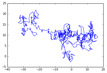
2. 模拟醉汉随机漫步

假设醉汉每一步的距离是1或2，方向也完全随机，360度不确定，然后模拟醉汉的行走路径.

我们用坐标表示醉汉的位置,每次产生两个随机数，一个是步长，就是醉汉一步走多远，我们假设1或2，r = np.random.randint(1,3,N),一个是方向，是一个度数，0-360,theta = np.radians(np.random.randint(0,361,N)),注意转化为弧度，每走一步，坐标值就是之前坐标值之和，用cumsum函数可以很方便地实现，x = np.cumsum(r*np.cos(theta)),y = np.cumsum(r*np.sin(theta))。然后ok了，plot一下看看醉汉的步伐有多醉人。

N = 500 # steps

r = np.random.randint(1,3,N) # move 1 or 2 units of distance each step
theta = np.radians(np.random.randint(0,361,N))

# np.cumsum Return the cumulative sum of the elements along a given axis.
x = np.cumsum(r*np.cos(theta))
y = np.cumsum(r*np.sin(theta))
plt.plot(x,y);

3. 使用梯形法计算一二次函数的数值积分

$\int_{a}^{b}f(x)dx$ we can partition the integration interval $[a,b]$ into smaller subintervals, and approximate the area under the curve for each subinterval by the area of the trapezoid created by linearly interpolating between the two function values at each end of the subinterval: 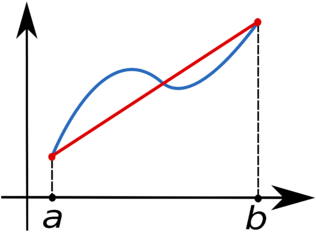The blue line represents the function $f(x)$ and the red line is the linear interpolation. By subdividing the interval $[a,b]$, the area under $f(x)$ can thus be approximated as the sum of the areas of all the resulting trapezoids.

If we denote by $x{i}$ ($i=0,\ldots,n,$ with $x{0}=a$ and $x_{n}=b$) the abscissas where the function is sampled, then

$\int_{a}^{b}f(x)dx\approx\frac{1}{2}\sum_{i=1}^{n}\left(x_{i}-x_{i-1}\right)\left(f(x_{i})+f(x_{i-1})\right).$

The common case of using equally spaced abscissas with spacing $h=(b-a)/n$ reads simply

$\int_{a}^{b}f(x)dx\approx\frac{h}{2}\sum_{i=1}^{n}\left(f(x_{i})+f(x_{i-1})\right).$ 具体计算只需要这个公式 $积分$ 道理很简单，就是把积分区间分割为很多小块，用梯形替代，其实还是局部用直线近似代替曲线的思想。这里对此一元二次函数积分，并与python模块积分制对比(精确值为4.5)用以验证。 $\int_a^b (x^2 - 3x + 2) dx$

from scipy import integrate
def f(x):
    return x*x - 3*x + 2

def trape(f,a,b,n=100):
    f = np.vectorize(f) # can apply on vector
    h = float(b - a)/n
    arr = f(np.linspace(a,b,n+1))
    return (h/2.)*(2*arr.sum() - arr[0] - arr[-1])

def quad(f,a,b):
    return integrate.quad(f,a,b)[0] # compare with python library result

a, b = -1, 2
print trape(f,a,b)
print quad(f,a,b)

4.50045
4.5

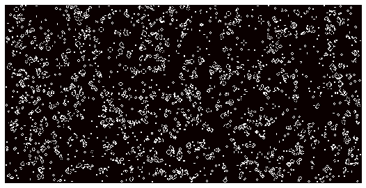
4. 模拟生命

模拟生命类似一个小游戏，可以假设有很多个小生命，或小细胞，可生可灭，具体k看这个细胞邻居的多少，规则如下,更多参见：

The universe of the Game of Life is an infinite two-dimensional orthogonal grid of square cells, each of which is in one of two possible states, live or dead. Every cell interacts with its eight neighbours, which are the cells that are directly horizontally, vertically, or diagonally adjacent. At each step in time, the following transitions occur:

Any live cell with fewer than two live neighbours dies, as if by needs caused by underpopulation.

Any live cell with more than three live neighbours dies, as if by overcrowding.

Any live cell with two or three live neighbours lives, unchanged, to the next generation.

Any dead cell with exactly three live neighbours becomes a live cell.

The initial pattern constitutes the 'seed' of the system. The first generation is created by applying the above rules simultaneously to every cell in the seed – births and deaths happen simultaneously, and the discrete moment at which this happens is sometimes called a tick. (In other words, each generation is a pure function of the one before.) The rules continue to be applied repeatedly to create further generations.

目标就是根据这些规则，确定经过若干次演变后，生命的形态，哪些细胞生，哪些细胞灭。例如：

Z = np.array([[0,0,0,0,0,0],
              [0,0,0,1,0,0],
              [0,1,0,1,0,0],
              [0,0,1,1,0,0],
              [0,0,0,0,0,0],
              [0,0,0,0,0,0]])

演变后就是

array([[0, 0, 0, 0, 0, 0],
       [0, 0, 0, 1, 0, 0],
       [0, 0, 0, 0, 1, 0],
       [0, 0, 1, 1, 1, 0],
       [0, 0, 0, 0, 0, 0],
       [0, 0, 0, 0, 0, 0]])

算法的关键是确定每个细胞的邻居多少，以决定生死，且假定边界均死，用0表示。

def evolve(Z):
    N = (Z[0:-2,0:-2] + Z[0:-2,1:-1] + Z[0:-2,2:] +
         Z[1:-1,0:-2]                + Z[1:-1,2:] +
         Z[2:  ,0:-2] + Z[2:  ,1:-1] + Z[2:  ,2:])
    # Apply rules
    birth = (N==3) & (Z[1:-1,1:-1]==0) #若本来死，且邻居为3，则复活
    survive = ((N==2) | (N==3)) & (Z[1:-1,1:-1]==1) # 若本来活，且邻居为2 or 3，则幸存
    Z[...] = 0 # 重置为0
    Z[1:-1,1:-1][birth | survive] = 1 # 复活或幸存的置为1
    return Z

Z = np.random.randint(0,2,(256,512))
for i in range(100): evolve(Z)

# plot
size = np.array(Z.shape)
dpi = 72.0
figsize= size[1]/float(dpi),size[0]/float(dpi)
fig = plt.figure(figsize=figsize, dpi=dpi, facecolor="white")
fig.add_axes([0.0, 0.0, 1.0, 1.0], frameon=False)
plt.imshow(Z,interpolation='nearest', cmap=plt.cm.hot)
plt.xticks([]), plt.yticks([])
plt.show()

Numpy作业